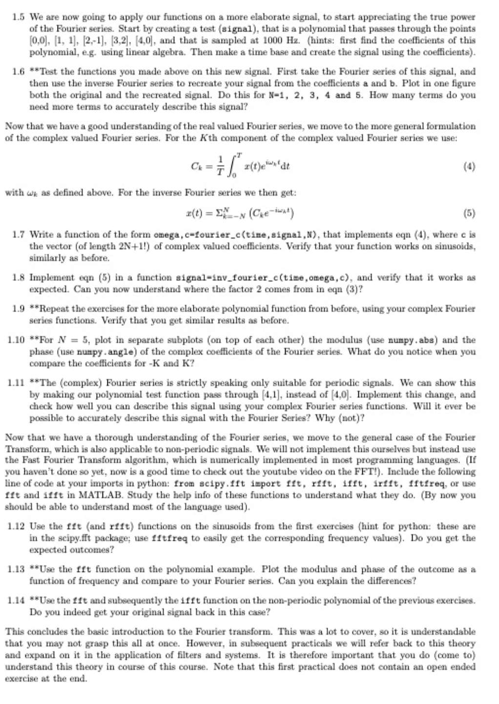
Computer practical $1$: intro to Fourier transforms$1\mathrm{.}5$ We are now going to apply our functions on a more elaborate signal, to start appreciating the true power

of the Fourier series. Start by creating a test $($signal$),$ that is a polynomial that passes through the points

$0,0$

$1,1$

$2,-1$

$3,2$

$4,0,$ and that is sampled at $1000Hz.($hints: first find the coefficients of this

polynomial, e$.$g$.$ using linear algebra. Then make a time base and create the signal using the coefficients$).$

${1\mathrm{.}6}^{****}$ Test the functions you made above on this new signal. First take the Fourier series of this signal, and

then use the inverse Fourier series to recreate your signal from the coefficients a and b$.$ Plot in one figure

both the original and the recreated signal. Do this for $N=1,2,3,4$ and $5.$ How many terms do you

need more terms to accurately describe this signal?

Now that we have a good understanding of the real valued Fourier series, we move to the more general formulation

of the complex valued Fourier series. For the $K$ th component of the complex valued Fourier series we use:

$C_k=\frac{1}{T}{\displaystyle \underset{0}{\overset{T}{}}}x(t)e^{i{}_{k}t}dt$

with ${}_k$ as defined above. For the inverse Fourier series we then get:

$x(t)={}_k=-N^N(C_k{e}^{-i{}_{}t})$

$1\mathrm{.}7$ Write a function of the form omega,c$-1$ourier$\_$c$($time$,$signal, $N),$ that implements eqn $(4),$ where $c$ is

the vector $($of length $2N+1!)$ of complex valued coefficients. Verify that your function works on sinusoids$,$

similarly as before.

$1\mathrm{.}8$ Implement eqn $(5)$ in a function signal$-$inv$\_$fourier$\_$c$($time$,$omega,c$),$ and verify that it works as

expected. Can you now understand where the factor $2$ comes from in eqn $(3)?$

${1\mathrm{.}9}^{****}$ Repeat the exercises for the more elaborate polynomial function from before, using your complex Fourier

series functions. Verify that you get similar results as before.

${1\mathrm{.}10}^{****}$ For $N=5,$ plot in separate subplots $($on top of each other$)$ the modulus $($use numpy. abs$)$ and the

phase $($use numpy $-$angle$)$ of the complex coefficients of the Fourier series. What do you notice when you

compare the coefficients for $-K$ and $K?$

${1\mathrm{.}11}^{****}$ The $($complex$)$ Fou

This assignment is intended to $1)$ refresh your programming and basic math skills and $2)$ to become acquainted

with Fourier transforms. We start with making some periodic test data, and applying the discrete Fourier series

to this. Then we'll compare our results to that of a Python or MATLAB implementation of the Fast Fourier

Transform, and explore some numerical properties thereof. We'll use the following real valued formulation of

the $($forward$)$ Fourier series $($only applicable to real valued signals$)$:

$A_k=\frac{1}{T}{\displaystyle \underset{0}{\overset{T}{}}}x(t)cos({}_{k}t)dt$

$B_k=\frac{1}{T}{\displaystyle \underset{0}{\overset{T}{}}}x(t)sin({}_{k}t)dt$

With ${}_k=\frac{2k}{T}$ and $T$ is the period time of the signal. This gives the following formulation for the $($inverse$)$

Fourier series:

$x(t)=A_0+2*{}_k=1^N(A_{k}cos({}_{k}t)+B_{k}sin({}_{k}t))$

where $N$ is the number of terms in the Fourier series $($can go up to infinity in the general case$).$

$1\mathrm{.}1$ Write a function to calculate the Fourier series for a real valued signal, based on the formulation in equa$-$

tions $(1)$ and $(2).$ the call to your function should look like this: omega $,$ a $,$ b$-$fourier$\_$ab$($time$,$signal,n$),$

where signal$($time$)$ describes the signal of which you take the Fourier series, and a and b are vectors of

length $N$ which are defined by the integrals in eqns $(1)$ and $(2).$

$1\mathrm{.}2$ Test your function by applying it $($separately$)$ to a sine and a cosine function of $1Hz$ with amplitude

First create the test signal over a time interval of $0,1,$ sampled at $100Hz.$ How many terms in

the Fourier series do you need to describe this signal? Do you get the expected outcome? Increase the

amplitude and frequency of the test signal and see if you get the expected outcomes in terms of a and b$.$

$1\mathrm{.}3$ Write a function to calculate the inverse Fourier series for a real valued signal, based on the formulation

in eqn $(3).$ The call to your function should look like this: signal$-$inv$\_$fourier$\_$ab$($time$,$ onega,a$,$b$),$

where the variables are defined similarly as above.

$1\mathrm{.}4$ Again test your function by inputting known values $($e$.$g$.$ the ones you created before$).$