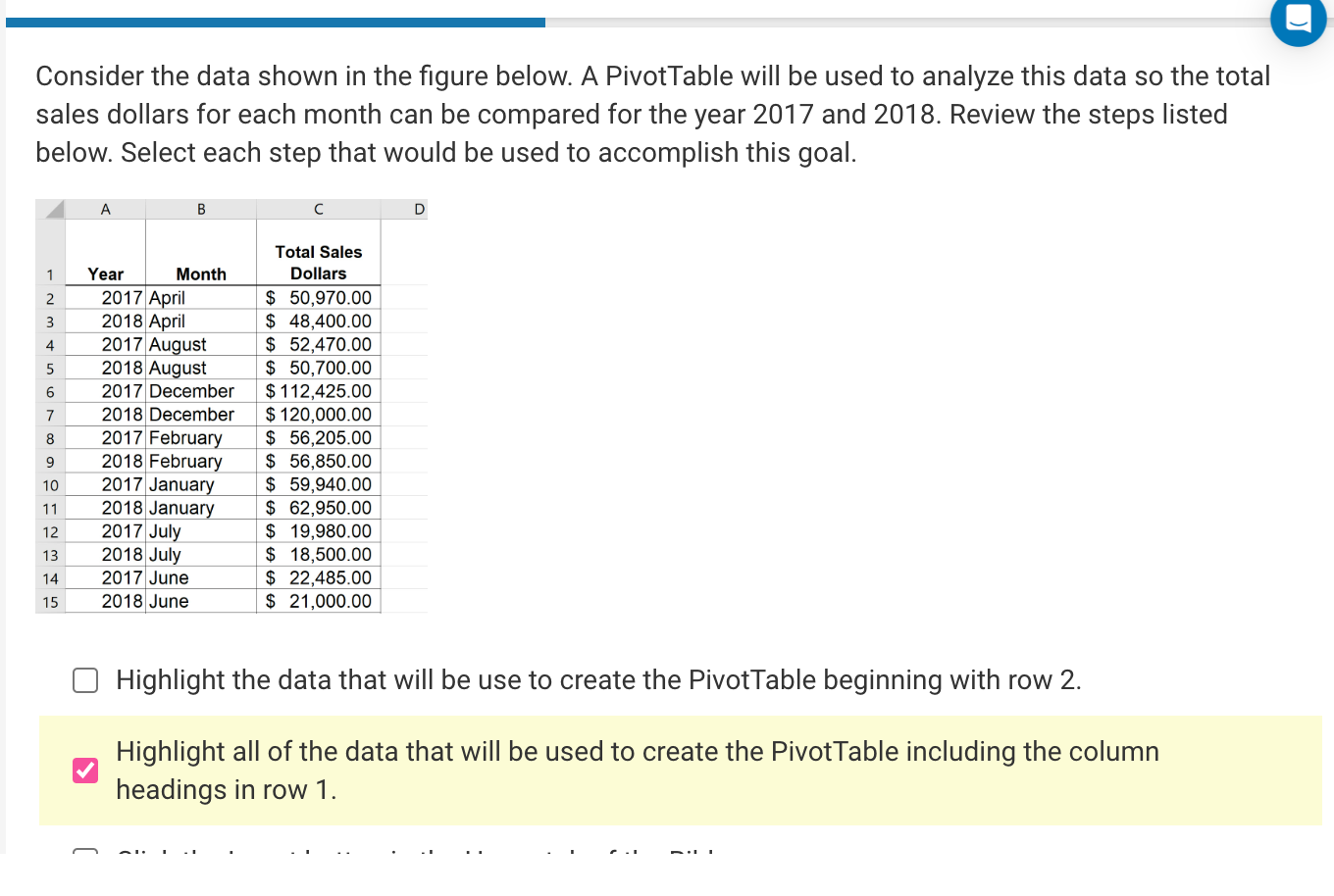
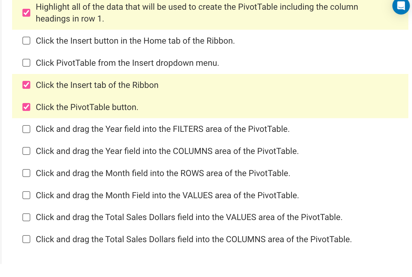
Consider the data shown in the figure below. A PivotTable will be used to analyze this data so the total sales dollars for each month can be compared for the year 2017 and 2018. Review the steps listed below. Select each step that would be used to accomplish this goal. Highlight the data that will be use to create the PivotTable beginning with row 2 . Highlight all of the data that will be used to create the PivotTable including the column headings in row 1 . Highlight all of the data that will be used to create the PivotTable including the column headings in row 1. Click the Insert button in the Home tab of the Ribbon. Click PivotTable from the Insert dropdown menu. Click the Insert tab of the Ribbon Click the PivotTable button. Click and drag the Year field into the FILTERS area of the PivotTable. Click and drag the Year field into the COLUMNS area of the PivotTable. Click and drag the Month field into the ROWS area of the PivotTable. Click and drag the Month Field into the VALUES area of the PivotTable. Click and drag the Total Sales Dollars field into the VALUES area of the PivotTable. Click and drag the Total Sales Dollars field into the COLUMNS area of the PivotTable. Consider the data shown in the figure below. A PivotTable will be used to analyze this data so the total sales dollars for each month can be compared for the year 2017 and 2018. Review the steps listed below. Select each step that would be used to accomplish this goal. Highlight the data that will be use to create the PivotTable beginning with row 2 . Highlight all of the data that will be used to create the PivotTable including the column headings in row 1 . Highlight all of the data that will be used to create the PivotTable including the column headings in row 1. Click the Insert button in the Home tab of the Ribbon. Click PivotTable from the Insert dropdown menu. Click the Insert tab of the Ribbon Click the PivotTable button. Click and drag the Year field into the FILTERS area of the PivotTable. Click and drag the Year field into the COLUMNS area of the PivotTable. Click and drag the Month field into the ROWS area of the PivotTable. Click and drag the Month Field into the VALUES area of the PivotTable. Click and drag the Total Sales Dollars field into the VALUES area of the PivotTable. Click and drag the Total Sales Dollars field into the COLUMNS area of the PivotTable