Consider the levered DCF model provided to you in tab A3 of the Excel spreadsheet.

Calculate the maximum price that an investor with the assumptions made in the model should be willing to pay for that property.

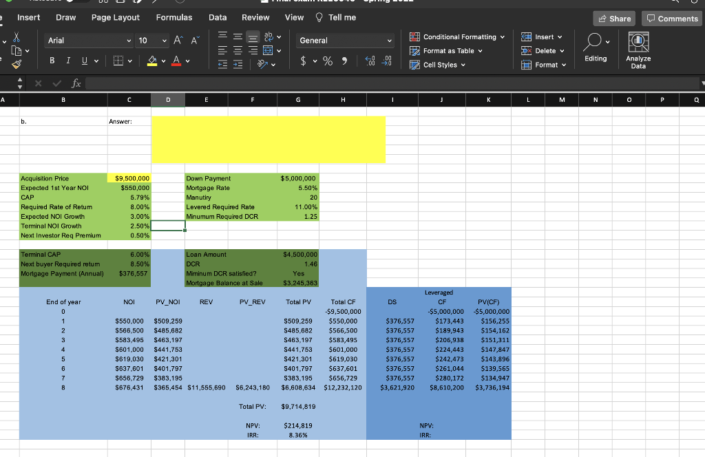
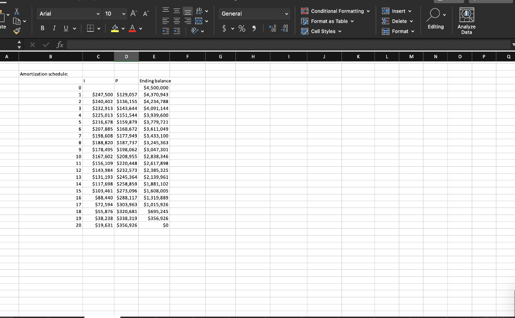
Insert Draw Page Layout Formulas Data Review View Tell me Share Comments Arial V 10 VAA = = = ab v General Insert v DX Delete v Conditional Formatting 12 Format as Table Cell Styles O @ Y V B I U v Av A V Editing $ % ) Y Format v Analyze Data X fx A B D E F H J K L M N 0 P Q b. Answer: Acquisition Price Expected 1st Year NOI CAP Required Rate of Retum Expected NOI Growth Terminal NOI Growth Next Investor Req Premium $9,500,000 $550,000 5.79% 8.00% 3.00% Down Payment Mortgage Rate Manutiry Levered Required Rate Minumum Required DCR $5,000,000 5.50% 20 11.00% 1.25 2.50% 0.50% Terminal CAP Next buyer Required retum Mortgage Payment (Annual) 6.00% 8.50% $376,557 Loan Amount DCR Miminum DCR satisfied? Mortgage Balance at Sale $4.500.000 1.46 Yes $3,245,363 NOI PV_NOI REV PV_REV DS End of year 0 1 2 3 $550.000 $566,500 $583,495 $601,000 $619.030 $637,601 $656,729 $676,431 Total PV Total CF -$9,500,000 S509,259 $550,000 S485,682 $566,500 $463.197 $583,495 $441,753 $601,000 S421.301 $619,030 S401.797 $637,601 S383,195 $656,729 $6,608,634 $12,232,120 $509,259 $485,682 $463,197 $441.753 $421.301 $401.797 $383,195 $365,454 $11,555,690 4 Leveraged CF $5,000,000 $173,443 $189,943 $206,938 $224,443 $242,473 $261,044 $280,172 $8,610,200 $376,557 $376,557 $376,557 $376,557 $376,557 $376,557 $376,557 $3,621,920 PV(CF) $5,000,000 $156,255 $154,162 $151,311 $147,847 $143,896 $139,565 $134,947 $3,736,194 5 6 7 $6,243,180 Total PV: $9,714,819 NPV: IRR: $214,819 8.36% NPV: IRR: Arial 10 v Insert v X [D ' A = = = ab General Conditional Formatting Format as Table v Cell Styles O FO M Analyze Data ste B I U A~ $ %) $ X Delete Format v Follo Editing Y 2.0 fx B C D E F G H I J L M N 0 P Q Amortization schedule: 1 1 0 1 2 3 4 5 6 7 8 9 10 P P Ending balance $4,500,000 $247,500 $129,057 $4,370,943 $240,402 $136,155 $4,234,788 $ 232,913 $143,644 $4,091,144 $225,013 $151,544 $3,939,600 $216,678 $159,879 $3,779,721 $207,885 $168,672 $3,611,049 $198,608 $177,949 $3,433,100 $188,820 $187,737 $3,245,363 $178,495 $198,062 $3,047,301 $167,602 $208,955 $2,838,346 $156,109 $220,448 $2,617,898 $143,984 $232,573 $2,385,325 $131,193 $245,364 $2,139,961 $117,698 $258,859 $1,881,102 $103,461 $273,096 $1,608,005 $88,440 $288,117 $1,319,889 $72,594 $303,963 $1,015,926 $55,876 $320,681 $695,245 $38,238 $338,319 $356,926 $19,631 $356,926 $0 11 12 13 14 15 16 17 18 19 20