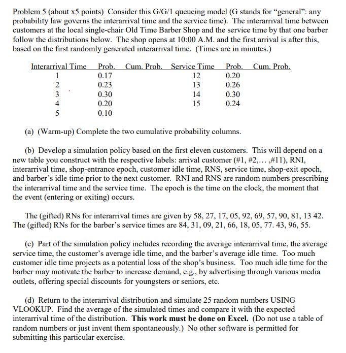
Consider this G/G/1 queueing model (G stands for general: any probability law governs the interarrival time and the service time). The interarrival time between customers at the local single-chair Old Time Barber Shop and the service time by that one barber follow the distributions below. The shop opens at 10:00 A.M. and the first arrival is after this, based on the first randomly generated interarrival time. (Times are in minutes.)

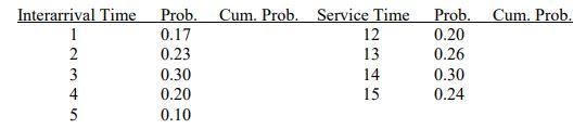
(a) (Warm-up) Complete the two cumulative probability columns.

(b) Develop a simulation policy based on the first eleven customers. This will depend on a new table you construct with the respective labels: arrival customer (#1, #2, ,#11), RNI, interarrival time, shop-entrance epoch, customer idle time, RNS, service time, shop-exit epoch, and barbers idle time prior to the next customer. RNI and RNS are random numbers prescribing the interarrival time and the service time. The epoch is the time on the clock, the moment that the event (entering or exiting) occurs. The (gifted) RNs for interarrival times are given by 58, 27, 17, 05, 92, 69, 57, 90, 81, 13 42. The (gifted) RNs for the barbers service times are 84, 31, 09, 21, 66, 18, 05, 77. 43, 96, 55.

(c) Part of the simulation policy includes recording the average interarrival time, the average service time, the customers average idle time, and the barbers average idle time. Too much customer idle time projects as a potential loss of the shops business. Too much idle time for the barber may motivate the barber to increase demand, e.g., by advertising through various media outlets, offering special discounts for youngsters or seniors, etc. (d) Return to the interarrival distribution and simulate 25 random numbers USING VLOOKUP. Find the average of the simulated times and compare it with the expected interarrival time of the distribution. This work must be done on Excel.

(Do not use a table of random numbers or just invent them spontaneously.) No other software is permitted for submitting this particular exercise

Cum. Prob. Interarrival Time 1 2 3 4 5 UN Prob. Cum. Prob. Service Time 0.17 12 0.23 13 0.30 14 0.20 15 0.10 Prob. 0.20 0.26 0.30 0.24 Problem 5 (about x5 points) Consider this G/G/1 queueing model (G stands for general: any probability law governs the interarrival time and the service time). The interarrival time between customers at the local single-chair Old Time Barber Shop and the service time by that one barber follow the distributions below. The shop opens at 10:00 A.M. and the first arrival is after this, based on the first randomly generated interarrival time. (Times are in minutes.) Interarrival Time Prob. Cum. Prob. Service Time Prob. Cum. Prob. 1 0.17 0.20 2 0.23 13 0.26 3 0.30 14 0.30 4 0.20 15 0.24 5 0.10 12 (a) (Warm-up) Complete the two cumulative probability columns. (6) Develop a simulation policy based on the first eleven customers. This will depend on a new table you construct with the respective labels: arrival customer (#1, #2,... #11), RNI, interarrival time, shop-entrance epoch, customer idle time, RNS, service time, shop-exit epoch, and barber's idle time prior to the next customer. RNI and RNS are random numbers prescribing the interarrival time and the service time. The epoch is the time on the clock, the moment that the event (entering or exiting) occurs. The (gifted) RNs for interarrival times are given by 58, 27, 17,05, 92, 69, 57, 90, 81, 13 42. The (gifted) RNs for the barber's service times are 84, 31, 09, 21, 66, 18, 05, 77. 43, 96, 55. (c) Part of the simulation policy includes recording the average interarrival time, the average service time, the customer's average idle time, and the barber's average idle time. Too much customer idle time projects as a potential loss of the shop's business. Too much idle time for the barber may motivate the barber to increase demand, e.g., by advertising through various media outlets, offering special discounts for youngsters or seniors, etc. (d) Return to the interarrival distribution and simulate 25 random numbers USING VLOOKUP. Find the average of the simulated times and compare it with the expected interarrival time of the distribution. This work must be done on Excel. (Do not use a table of random numbers or just invent them spontaneously.) No other software is permitted for submitting this particular exercise. Cum. Prob. Interarrival Time 1 2 3 4 5 UN Prob. Cum. Prob. Service Time 0.17 12 0.23 13 0.30 14 0.20 15 0.10 Prob. 0.20 0.26 0.30 0.24 Problem 5 (about x5 points) Consider this G/G/1 queueing model (G stands for general: any probability law governs the interarrival time and the service time). The interarrival time between customers at the local single-chair Old Time Barber Shop and the service time by that one barber follow the distributions below. The shop opens at 10:00 A.M. and the first arrival is after this, based on the first randomly generated interarrival time. (Times are in minutes.) Interarrival Time Prob. Cum. Prob. Service Time Prob. Cum. Prob. 1 0.17 0.20 2 0.23 13 0.26 3 0.30 14 0.30 4 0.20 15 0.24 5 0.10 12 (a) (Warm-up) Complete the two cumulative probability columns. (6) Develop a simulation policy based on the first eleven customers. This will depend on a new table you construct with the respective labels: arrival customer (#1, #2,... #11), RNI, interarrival time, shop-entrance epoch, customer idle time, RNS, service time, shop-exit epoch, and barber's idle time prior to the next customer. RNI and RNS are random numbers prescribing the interarrival time and the service time. The epoch is the time on the clock, the moment that the event (entering or exiting) occurs. The (gifted) RNs for interarrival times are given by 58, 27, 17,05, 92, 69, 57, 90, 81, 13 42. The (gifted) RNs for the barber's service times are 84, 31, 09, 21, 66, 18, 05, 77. 43, 96, 55. (c) Part of the simulation policy includes recording the average interarrival time, the average service time, the customer's average idle time, and the barber's average idle time. Too much customer idle time projects as a potential loss of the shop's business. Too much idle time for the barber may motivate the barber to increase demand, e.g., by advertising through various media outlets, offering special discounts for youngsters or seniors, etc. (d) Return to the interarrival distribution and simulate 25 random numbers USING VLOOKUP. Find the average of the simulated times and compare it with the expected interarrival time of the distribution. This work must be done on Excel. (Do not use a table of random numbers or just invent them spontaneously.) No other software is permitted for submitting this particular exercise