Create a PivotTable.

a$.$ Select cell A$5$ and click the Table Name box $[$Table tab, Properties group$].$

b$.$ Name the table tblHours.

c$.$ Click the Summarize with PivotTable button $[$Table tab, Tools group$].$ The range is identified as tb$/$Hours$.$

d$.$ Verify that New Worksheet is selected and click OK$.$

e$.$ Name the sheet PivotTable.

Manage fields in a PivotTable.

a$.$

Show the Product$/$Service and Billable fields in the PivotTable.

b$.$

Drag the Billable field from the Field Name area below the Sum of Billable field in the Values area so

that it appears twice in the report layout and the pane.

c$.$

Select cell C$4$ and open the Value Field Settings dialog box. NOTE: You can select any cell in column C

within the PivotTable data in order to complete the following steps to modify the PivotTable column

settings.

d$.$ Type Average Hours as the Custom Name, choose Average as the calculation, and set the Number

Format to Number with two decimal places.

e$.$

Select cell B$4$ and open the Value Field Settings dialog box. Set its Custom Name to Tchal Hours and

the number format to Number with two decimal places.

f$.$

Apply Dark Gray, Pivot Style Dark $11$ with banded rows and columns.

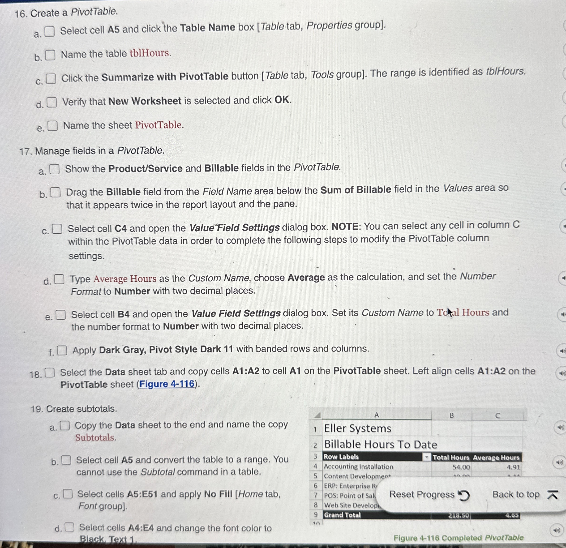
Select the Data sheet tab and copy cells A$1$:A$2$ to cell A$1$ on the PivotTable sheet. Left align cells A$1$:A$2$ on the

PivotTable sheet $($Figure $4-116).$

Create subtotals.

a$.$

Copy the Data sheet to the end and name the copy

Subtotals.

b$.$

Select cell A$5$ and convert the table to a range. You

cannot use the Subtotal command in a table.

c$.$

Select cells A$5$:E$51$ and apply No Fill $[$Home tab,

Font group$].$

d$.$ Select cells A$4$:E$4$ and change the font color to

Black. Text $1.$