1. Create a single variable data table to determine the impact that the variable interest rates (in the range A12:A22) will have on the total cost of the campground.
   1. In cell B11, create a formula without using a function that references cell D5 (the monthly payments).
   2. In cell C11, create a formula without using a function that references cell D6 (the total interest paid on the loan).
   3. In cell D11, create a formula without using a function that references cell D7 (the total cost of the mortgage).
   4. Select the range A11:D26 and create a single-variable data table, using an absolute reference to cell D3 (the mortgage interest rate) as the Column input cell.
2. To help Kaleen identify how each rate in her Variable Interest Rate Schedule compares to the interest rate she anticipates on her mortgage, she decides to highlight the matching interest rate in the schedule with a conditional formatting rule.

Apply a Highlight Cells conditional formatting rule to the range A12:A26 that formats any cell in the range that is equal to the value in cell D3 (using an absolute reference to cell D3) with Green Fill with Dark Green Text.

3. Kaleen now wishes to finalize the Amortization schedule.

In cell J4, create a formula without using a function that subtracts the value in cell I4 from the value in cell H4 to determine how much of the mortgage principal is being paid off each year.

Copy the formula in cell J4 to the range J5:J18.

4. In cell K4, create a formula using the IF function to calculate the interest paid on the mortgage (or the difference between the total payments made each year and the total amount of mortgage principal paid each year).
   1. The formula should first check if the value in cell H4 (the balance remaining on the loan each year) is greater than 0.
   2. If the value in cell H4 is greater than 0, the formula should return the value in J4 subtracted from the value in cell D5 multiplied by 12. Use a relative cell reference to cell J4 and an absolute cell reference to cell D5. (Hint: Use 12*$D$5-J4 as the is_true argument value in the formula.)
   3. If the value in cell H4 is not greater than 0, the formula should return a value of 0.

Copy the formula from cell K4 into the range K5:K18.

5. Apply the Accounting number format with two decimal places and $ as the symbol to the range K4:K18.
6. In cell K20, create a formula without using a function that references the defined name Down_Payment.

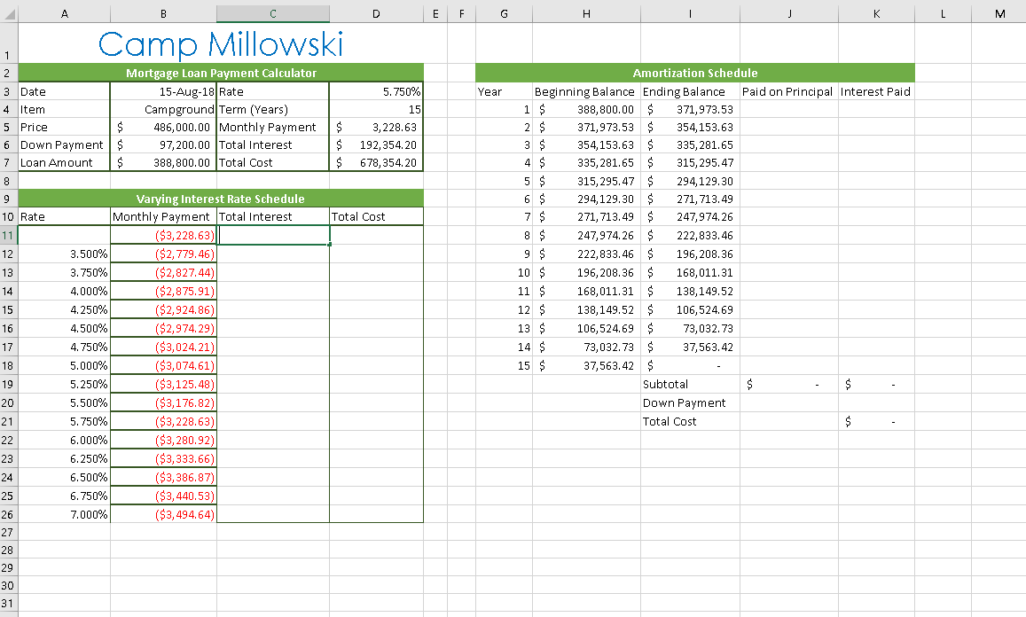
B D E F G H Camp Millowski Year Mortgage Loan Payment Calculator 3 Date 15-Aug-18 Rate 4 Item Campground Term (Years) 5 Price 486,000.00 Monthly Payment 6 Down Payment | $ 97,200.00 Total Interest 7 Loan Amount $ 388,800.00 Total Cost $ $ $ 5.750% 15 3,228.63 192,354.20 678,354.20 10 Rate Total Cost 3.500% 3.750% 4.000% 4.250% 4.500% 4.750% 5.000% 5.250% 5.500% 5.750% 6.000% 6.250% 6.500% 6.750% 7.000% Varying Interest Rate Schedule Monthly Payment Total Interest ($3,228.63) ($2,779.46) ($2,827.44) ($2,875.91) ($2,924.86) ($2,974.29) ($3,024.21) ($3,074.61) ($3,125.48) ($3,176.82) ($3,228.63) ($3,280.92) ($3,333.66) ($3,386.87) ($3,440.53) ($3,494.64)| Amortization Schedule Beginning Balance Ending Balance Paid on Principal Interest Paid 1 $ 388,800.00 $ 371,973.53 2 $ 371,973.53 $ 354,153.63 3 $ 354,153.63 $ 335,281.65 4 $ 335,281.65 $ 315,295.47 5 $ 315,295.47 $ 294,129.30 6 $ 294,129.30 $ 271, 713.49 271, 713.49 $ 247,974.26 247,974.26 $ 222,833.46 9 $ 222,833.46 $ 196,208.36 10 $ 196,208.36 $ 168,011.31 11 $ 168,011.31 $ 138,149.52 12 $ 138,149.52 $ 106,524.69 13 $ 106,524.69 $ 73,032.73 14 $ 73,032.73 $ 37,563.42 15 $ 37,563.42 $ Subtotal Down Payment Total Cost B D E F G H Camp Millowski Year Mortgage Loan Payment Calculator 3 Date 15-Aug-18 Rate 4 Item Campground Term (Years) 5 Price 486,000.00 Monthly Payment 6 Down Payment | $ 97,200.00 Total Interest 7 Loan Amount $ 388,800.00 Total Cost $ $ $ 5.750% 15 3,228.63 192,354.20 678,354.20 10 Rate Total Cost 3.500% 3.750% 4.000% 4.250% 4.500% 4.750% 5.000% 5.250% 5.500% 5.750% 6.000% 6.250% 6.500% 6.750% 7.000% Varying Interest Rate Schedule Monthly Payment Total Interest ($3,228.63) ($2,779.46) ($2,827.44) ($2,875.91) ($2,924.86) ($2,974.29) ($3,024.21) ($3,074.61) ($3,125.48) ($3,176.82) ($3,228.63) ($3,280.92) ($3,333.66) ($3,386.87) ($3,440.53) ($3,494.64)| Amortization Schedule Beginning Balance Ending Balance Paid on Principal Interest Paid 1 $ 388,800.00 $ 371,973.53 2 $ 371,973.53 $ 354,153.63 3 $ 354,153.63 $ 335,281.65 4 $ 335,281.65 $ 315,295.47 5 $ 315,295.47 $ 294,129.30 6 $ 294,129.30 $ 271, 713.49 271, 713.49 $ 247,974.26 247,974.26 $ 222,833.46 9 $ 222,833.46 $ 196,208.36 10 $ 196,208.36 $ 168,011.31 11 $ 168,011.31 $ 138,149.52 12 $ 138,149.52 $ 106,524.69 13 $ 106,524.69 $ 73,032.73 14 $ 73,032.73 $ 37,563.42 15 $ 37,563.42 $ Subtotal Down Payment Total Cost