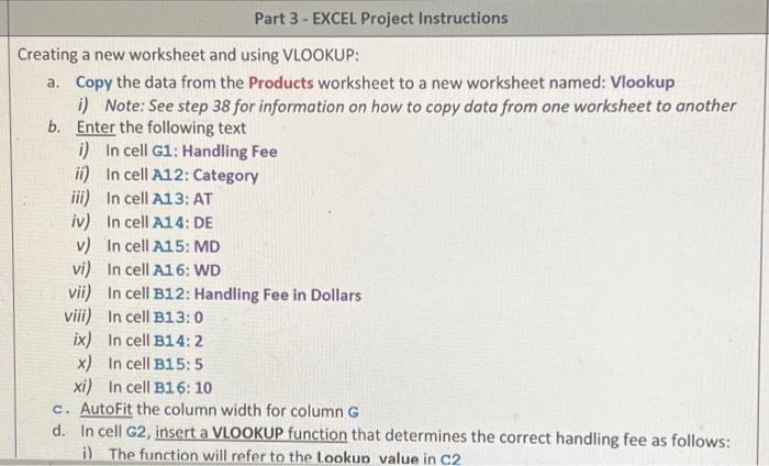
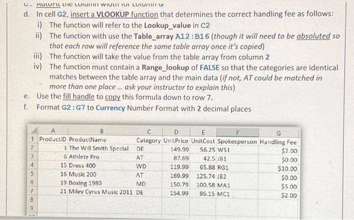
Creating a new worksheet and using VLOOKUP: a. Copy the data from the Products worksheet to a new worksheet named: Vlookup i) Note: See step 38 for information on how to copy data from one worksheet to another b. Enter the following text i) In cell G1: Handling Fee ii) In cell A12: Category iii) In cell A13: AT iv) In cell A14:DE v) In cell A15: MD vi) In cell A16: WD vii) In cell B12: Handling Fee in Dollars viii) In cell B13:0 ix) In cell B14:2 x) In cell B15:5 xi) In cell B16: 10 c. AutoFit the column width for column G d. In cell G2, insert a VLOOKUP function that determines the correct handling fee as follows: d. In cell G2, insert a VLOOKUP function that determines the correct handling fee as follows: i) The function will refer to the Lookup_value in C2 ii) The function with use the Table_array A12 : B16 (though it will need to be absoluted so that each row will reference the same table array once it's copied) iii) The function will take the value from the table array from column 2 iv) The function must contain a Range_lookup of FALSE so that the categories are identical matches between the table array and the main data (if not, AT could be matched in more than one place... ask your instructor to explain this) e. Use the fill handle to copy this formula down to row 7. f. Format G2: G7 to Currency Number Format with 2 decimal places