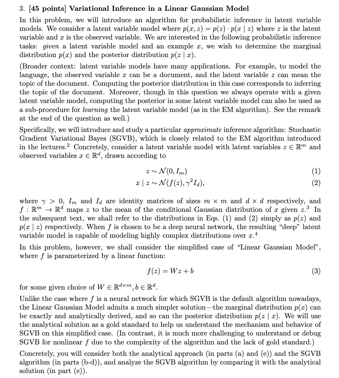
CS229 Problem Set #3 9 (a) [5 points] Exact marginal inference. By exploiting the linearity of f, we will first show that p(x) can be determined analytically. We shall do so by explicitly finding a closed-form expression for p(x). To begin, we make the following observation: letting o ~ N(0, 72Id), we can see that the process for generating x is the same as x = Wz+b+d. (4) Since z and o are Gaussian random variables, x must also be a Gaussian random variable. Thus, p(x) must be a Gaussian distribution N(v, I) for some choice of mean vector v E R and covariance matrix D e Rdxd, where I' is symmetric and positive definite. Task: Express v and I as functions of (W, b, y). You do not need to prove that x is a Gaussian random variable or that p(x) is a Gaussian distribution in your answer; you only need to provide expressions for v and I. Hint: By definition of the Gaussian distribution parameters, v = E[x] and I = cov(x). (b) [5 points] Understanding the ELBO. From Q3a, we see that we can exploit the linearity of f to determine In p(x) analytically. In general, however, exact calculation of Inp(x) is often intractable, and we must develop methods to instead approximate Inp(x). One such method is variational inference, which converts the estimation of In p(x) into an optimization problem by using the Evidence Lower Bound (ELBO), ELBO(x; q) = EzNg In P(2, z) q(z) (5) where q is some choice of distribution over the space of z. Note that in the equation above q(t) denotes the density of q at t, and z ~ q means a random variable z is sampled from the distribution of q. Crucially, as shown in the lecture, the ELBO always lower bounds In p(x), In p(x) > ELBO(x; q) = EzNg In P(2, 2) q(z) (6) no matter what choice of q you use. Since this bound holds for any choice of q, we can approximate In p(x) by optimizing q over some space of distributions 2, In p(x) 2 max ELBO(x; q), (7) so that the ELBO is as large as possible (thus giving the best approximation for In p(x)). We refer to Q as the variational family, and each q E 2 as a proposal or variational distribution. Before we discuss how to optimize the ELBO, let us briefly familiarize ourselves with the ELBO by considering two decompositions of the ELBO that exposes its relation to the Kullback-Leibler (KL) divergence. i. Task: Prove that ELBO(x; q) = Ez~q Inp(x | z) - DKL(q l| Pz). (8) ii. Task: Prove that ELBO(x; q) = Inp(x) - DKL(q || Pzz). (9)3. [45 points] Variational Inference in a Linear Gaussian Model In this problem, we will introduce an algorithm for probabilistic inference in latent variable models. We consider a latent variable model where p(:r, z) = p(z) op(:r | 2:) where z is the latent variable and a: is the observed variable. We are interested in the following probabilistic inference tasks; given a latent variable model and an example as, we wish to determine the marginal distribution 30(3) and the posterior distribution p(z | at). (Broader context: latent variable models have many applications. For example, to model the language, the observed variable a: can be a document, and the latent variable 2 can mean the topic of the document. Computing the posterior distribution in this case corresponds to inferring the topic of the document. Moreover, though in this question we always operate with a given latent variable model, computing the posterior in some latent variable model can also be used as a sub-procedure for learning the latent variable model (as in the EM algorithm). See the remark at the end of the question as well.) Specically, we will introduce and study a particular approximate inference algorithm: Stochastic Gradient Variational Bayes (SGVB), which is closely related to the EM algorithm introduced in the lectures.2 Concretely, consider a latent variable model with latent variables 2: E Em and observed variables a: 6 Rd, drawn according to 2: ~ N(0,Im) (1) 3!: I z N N(f(z)1T2Id)= (2) where \"y > 0, Im and Id are identity matrices of sizes m x m and d x (1 respectively, and f : Rm ) Rd maps 2 to the mean of the conditional Gaussian distribution of a: given 2.3 In the subsequent text, we shall refer to the distributions in Eqs. (1) and (2) simply as 30(3) and p(a: | z) respectively. When f is chosen to be a deep neural network, the resulting \"deep\" latent variable model is capable of modeling highly complex distributions over 13.4 In this problem, however, we shall consider the simplied case of \"Linear Gaussian Model\