csv file

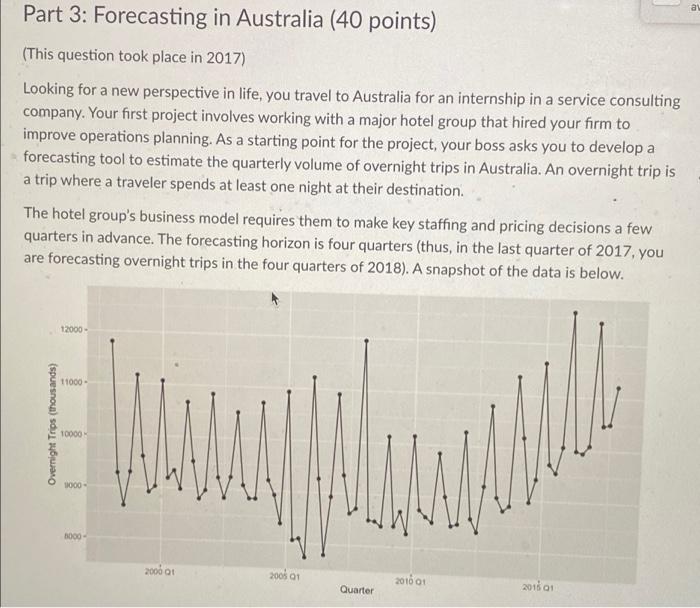
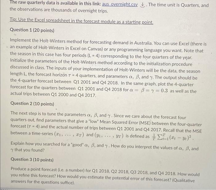
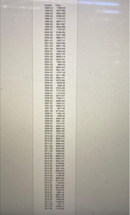
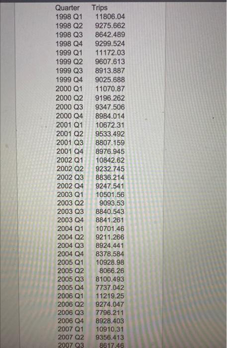
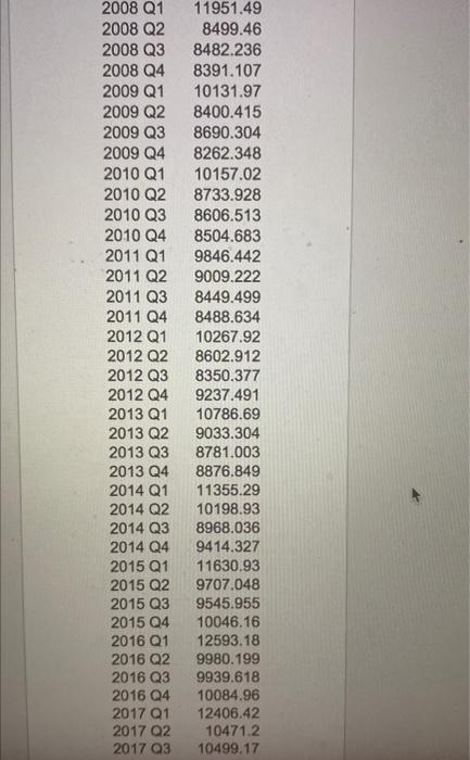
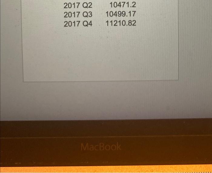
al Part 3: Forecasting in Australia (40 points) (This question took place in 2017) Looking for a new perspective in life, you travel to Australia for an internship in a service consulting company. Your first project involves working with a major hotel group that hired your firm to improve operations planning. As a starting point for the project, your boss asks you to develop a forecasting tool to estimate the quarterly volume of overnight trips in Australia. An overnight trip is a trip where a traveler spends at least one night at their destination. The hotel group's business model requires them to make key staffing and pricing decisions a few quarters in advance. The forecasting horizon is four quarters (thus, in the last quarter of 2017, you are forecasting overnight trips in the four quarters of 2018). A snapshot of the data is below. 12000 11000 Overnight Trips (thousands) 10000 will 1000- 2000- 2000 01 2005 01 201601 Quarter 201501 The raw quarterly data is available in this link: aus overnight.csv The time unit is Quarters, and the observations are thousands of overnight trips. Tip: Use the Excel spreadsheet in the forecast module as a starting point Question 1 (20 points) Implement the Holt-Winters method for forecasting demand in Australia. You can use Excel (there is an example of Holt-Winters in Excel on Canvas) or any programming language you want. Note that the season in this case has four periods (L = 4) corresponding to the four quarters of the year. Initialize the parameters of the Holt-Winters method according to the initialization procedure discussed in class. The inputs of your implementation of Holt-Winters will be the data, the season length L, the forecast horizon T = 4 quarters, and parameters a, b, and y. The output should be the 4-quarter forecast between Q1 2001 and Q4 2018. In the same graph, plot the 4-quarter forecast for the quarters between Q1 2001 and Q4 2018 for a = B =y=0.3 as well as the actual trips between Q1 2000 and Q4 2017. Question 2 (10 points) The next step is to tune the parameters a, b, and y. Since we care about the forecast four quarters out, find parameters that give a "low" Mean Squared Error (MSE) between the four-quarter forecast T = 4) and the actual number of trips between Q1 2001 and Q4 2017. Recall that the MSE between a time-series (21, ... , r) and (91, ..., yr) is defined as ? (x - y). Explain how you searched for a "good" a, b, and y. How do you interpret the values of a, b, and y that you found? Question 3 (10 points) Produce a point forecast (i.e. a number) for Q1 2018, Q2 2018, Q3 2018, and Q4 2018. How would you refine this forecast? How would you estimate the potential error of this forecast? (Qualitative answers for the questions suffice). 2016 D Quan 18 ! 1180 100 275.0 100003 200 19000 2004 100001 11723 100002 000T 813 100003 2013 1994 9025 2000 01 11070 BY 2000 2 20003 347 500 20004 2014 2001 01 1087231 2001 33.0 2001 03 07150 2001 04 007. 2002 01 10022 200203 232.1 2002 03 214 2002 01 9947541 2003 01 10501 Se 2003 02 2003 2003 05 5840 641201 200401 1010140 2004 9211.200 2004 200404 BOT 2005: 10926 2005 806620 2005 Q3 0100,400 2005 7737.32 2006 01 1121925 ES YO COOR COM 20002 200000 RUE 7790.215 880.00 10010 2007 01 w 2007 2007 9906 2007 1011 1740 1716.350 M 6423 10918 100415 YO 2006 01 2000 2008 20000 2000 2 200003 20000 2010: 2010 02 ONS 2009 DKK NOUS WA 06.13 DON 9000 222 SA 100870 2011 2012 2011 09 2011 ok 201203 201203 20120 201303 2013 201504 2012 200 ut ce VOICE 00 100 2013 2 TO COM CO EN 70 TO BE 1010 w 2014 2010 2011 20001 103 BORSE 2018 2018 2017 2017 2019 20 16 Quarter Trips 1998 Q1 11806.04 1998 Q2 9275.662 1998 Q3 8642.489 1998 Q4 9299.524 1999 Q1 11172.03 1999 Q2 9607.613 1999 Q3 8913.887 1999 Q4 9025.688 2000 Q1 11070.87 2000 Q2 9196.262 2000 Q3 9347.506 2000 Q4 8984.014 2001 Q1 10672.31 2001 Q2 9533.492 2001 Q3 8807.159 2001 Q4 8976.945 2002 Q1 10842.62 2002 Q2 9232.745 2002 Q3 8836.214 2002 Q4 9247.541 2003 01 10501.56 2003 Q2 9093.53 2003 Q3 8840.543 2003 Q4 8841.261 2004 Q1 10701.46 2004 Q2 9211.266 2004 Q3 8924.441 2004 Q4 8378.584 2005 Q1 10928.98 2005 Q2 8066.26 2005 Q3 8100.493 2005 Q4 7737.042 2006 Q1 11219.25 2006 Q2 9274.047 2006 Q3 7796.211 2006 Q4 8928.403 2007 Q1 10910.31 2007 Q2 9356.413 2007 Q3 861746 2008 Q1 2008 Q2 2008 Q3 2008 Q4 2009 Q1 2009 Q2 2009 Q3 2009 Q4 2010 Q1 2010 Q2 2010 Q3 2010 Q4 2011 Q1 2011 Q2 2011 Q3 2011 Q4 2012 Q1 2012 Q2 2012 Q3 2012 Q4 2013 Q1 2013 Q2 2013 Q3 2013 Q4 2014 Q1 2014 Q2 2014 Q3 2014 Q4 2015 Q1 2015 Q2 2015 Q3 2015 Q4 2016 Q1 2016 Q2 2016 Q3 2016 Q4 2017 Q1 2017 Q2 2017 Q3 11951.49 8499.46 8482.236 8391.107 10131.97 8400.415 8690.304 8262.348 10157.02 8733.928 8606.513 8504.683 9846.442 9009.222 8449.499 8488.634 10267.92 8602.912 8350.377 9237.491 10786.69 9033.304 8781.003 8876.849 11355.29 10198.93 8968.036 9414.327 11630.93 9707.048 9545.955 10046.16 12593.18 9980.199 9939.618 10084.96 12406.42 10471.2 10499.17 2017 Q2 2017 Q3 2017 Q4 10471.2 10499.17 11210.82 MacBook al Part 3: Forecasting in Australia (40 points) (This question took place in 2017) Looking for a new perspective in life, you travel to Australia for an internship in a service consulting company. Your first project involves working with a major hotel group that hired your firm to improve operations planning. As a starting point for the project, your boss asks you to develop a forecasting tool to estimate the quarterly volume of overnight trips in Australia. An overnight trip is a trip where a traveler spends at least one night at their destination. The hotel group's business model requires them to make key staffing and pricing decisions a few quarters in advance. The forecasting horizon is four quarters (thus, in the last quarter of 2017, you are forecasting overnight trips in the four quarters of 2018). A snapshot of the data is below. 12000 11000 Overnight Trips (thousands) 10000 will 1000- 2000- 2000 01 2005 01 201601 Quarter 201501 The raw quarterly data is available in this link: aus overnight.csv The time unit is Quarters, and the observations are thousands of overnight trips. Tip: Use the Excel spreadsheet in the forecast module as a starting point Question 1 (20 points) Implement the Holt-Winters method for forecasting demand in Australia. You can use Excel (there is an example of Holt-Winters in Excel on Canvas) or any programming language you want. Note that the season in this case has four periods (L = 4) corresponding to the four quarters of the year. Initialize the parameters of the Holt-Winters method according to the initialization procedure discussed in class. The inputs of your implementation of Holt-Winters will be the data, the season length L, the forecast horizon T = 4 quarters, and parameters a, b, and y. The output should be the 4-quarter forecast between Q1 2001 and Q4 2018. In the same graph, plot the 4-quarter forecast for the quarters between Q1 2001 and Q4 2018 for a = B =y=0.3 as well as the actual trips between Q1 2000 and Q4 2017. Question 2 (10 points) The next step is to tune the parameters a, b, and y. Since we care about the forecast four quarters out, find parameters that give a "low" Mean Squared Error (MSE) between the four-quarter forecast T = 4) and the actual number of trips between Q1 2001 and Q4 2017. Recall that the MSE between a time-series (21, ... , r) and (91, ..., yr) is defined as ? (x - y). Explain how you searched for a "good" a, b, and y. How do you interpret the values of a, b, and y that you found? Question 3 (10 points) Produce a point forecast (i.e. a number) for Q1 2018, Q2 2018, Q3 2018, and Q4 2018. How would you refine this forecast? How would you estimate the potential error of this forecast? (Qualitative answers for the questions suffice). 2016 D Quan 18 ! 1180 100 275.0 100003 200 19000 2004 100001 11723 100002 000T 813 100003 2013 1994 9025 2000 01 11070 BY 2000 2 20003 347 500 20004 2014 2001 01 1087231 2001 33.0 2001 03 07150 2001 04 007. 2002 01 10022 200203 232.1 2002 03 214 2002 01 9947541 2003 01 10501 Se 2003 02 2003 2003 05 5840 641201 200401 1010140 2004 9211.200 2004 200404 BOT 2005: 10926 2005 806620 2005 Q3 0100,400 2005 7737.32 2006 01 1121925 ES YO COOR COM 20002 200000 RUE 7790.215 880.00 10010 2007 01 w 2007 2007 9906 2007 1011 1740 1716.350 M 6423 10918 100415 YO 2006 01 2000 2008 20000 2000 2 200003 20000 2010: 2010 02 ONS 2009 DKK NOUS WA 06.13 DON 9000 222 SA 100870 2011 2012 2011 09 2011 ok 201203 201203 20120 201303 2013 201504 2012 200 ut ce VOICE 00 100 2013 2 TO COM CO EN 70 TO BE 1010 w 2014 2010 2011 20001 103 BORSE 2018 2018 2017 2017 2019 20 16 Quarter Trips 1998 Q1 11806.04 1998 Q2 9275.662 1998 Q3 8642.489 1998 Q4 9299.524 1999 Q1 11172.03 1999 Q2 9607.613 1999 Q3 8913.887 1999 Q4 9025.688 2000 Q1 11070.87 2000 Q2 9196.262 2000 Q3 9347.506 2000 Q4 8984.014 2001 Q1 10672.31 2001 Q2 9533.492 2001 Q3 8807.159 2001 Q4 8976.945 2002 Q1 10842.62 2002 Q2 9232.745 2002 Q3 8836.214 2002 Q4 9247.541 2003 01 10501.56 2003 Q2 9093.53 2003 Q3 8840.543 2003 Q4 8841.261 2004 Q1 10701.46 2004 Q2 9211.266 2004 Q3 8924.441 2004 Q4 8378.584 2005 Q1 10928.98 2005 Q2 8066.26 2005 Q3 8100.493 2005 Q4 7737.042 2006 Q1 11219.25 2006 Q2 9274.047 2006 Q3 7796.211 2006 Q4 8928.403 2007 Q1 10910.31 2007 Q2 9356.413 2007 Q3 861746 2008 Q1 2008 Q2 2008 Q3 2008 Q4 2009 Q1 2009 Q2 2009 Q3 2009 Q4 2010 Q1 2010 Q2 2010 Q3 2010 Q4 2011 Q1 2011 Q2 2011 Q3 2011 Q4 2012 Q1 2012 Q2 2012 Q3 2012 Q4 2013 Q1 2013 Q2 2013 Q3 2013 Q4 2014 Q1 2014 Q2 2014 Q3 2014 Q4 2015 Q1 2015 Q2 2015 Q3 2015 Q4 2016 Q1 2016 Q2 2016 Q3 2016 Q4 2017 Q1 2017 Q2 2017 Q3 11951.49 8499.46 8482.236 8391.107 10131.97 8400.415 8690.304 8262.348 10157.02 8733.928 8606.513 8504.683 9846.442 9009.222 8449.499 8488.634 10267.92 8602.912 8350.377 9237.491 10786.69 9033.304 8781.003 8876.849 11355.29 10198.93 8968.036 9414.327 11630.93 9707.048 9545.955 10046.16 12593.18 9980.199 9939.618 10084.96 12406.42 10471.2 10499.17 2017 Q2 2017 Q3 2017 Q4 10471.2 10499.17 11210.82 MacBook