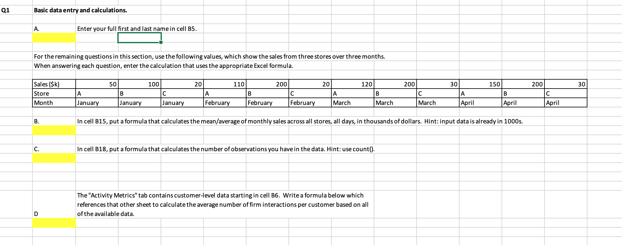
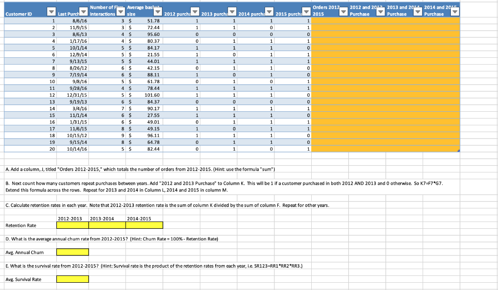
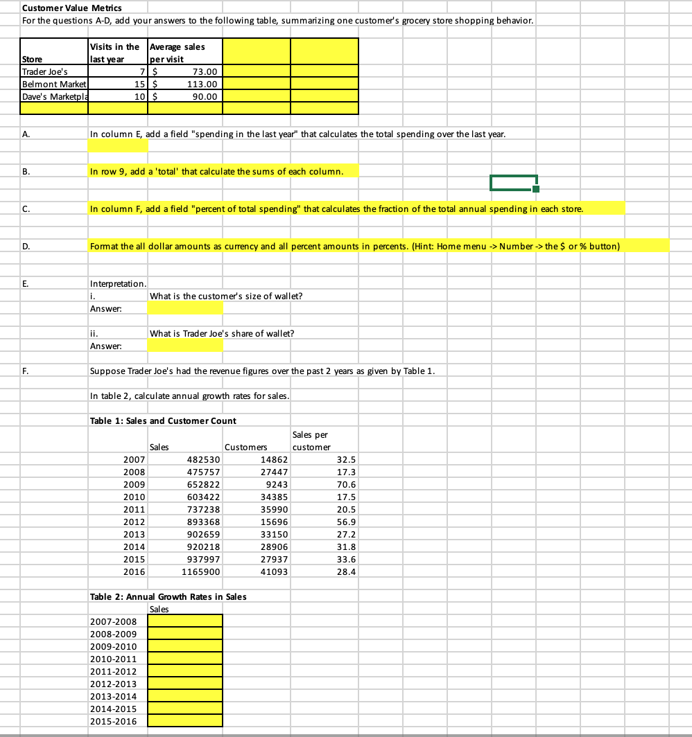
Customer Metrics Google Sheets Tutorial Customer Analytics - Professor Atlas Objectives of Today's Session - Introduction to Google Sheets: orientation, formulas, cell references - Calculate common traditional marketing, customer acquisition metrics in Google Sheets - This foundation will provide a foundation to use Google Sheets to calculate the customer metrics discussed in the video lecture Calculating Metrics Imagine that you are the director of customer analytics for TLC Coffee. You have been given some information and need to calculate the appropriate marketing metrics. You have been given the information in the data set "Applied Assignment 2 - Customer Metrics Data.xlsx" in the tab "Market Data." On behalf of TLC, here are your objectives: 1. You want to know the total sales, average sales and market share for each company, for each year. What is the market share of TLC and its rivals in 2017 and 2018? IMPORTANT: All of the steps below are to be completed in the data set worksheet titled "Applied Assignment 2- Customer Metrics Data" To do this, we'll need to first total up the sales across the market. Insert a row below row 7. What's a row? Google Sheets spreadsheets are organized as a series of columns and rows, on a series of worksheets. Columns are vertical, like wallpaper, and are lettered (A, B, C, ..). Rows are horizontal, like a shelf, and are numbered (1,2,3,). Worksheets are tabbed at the bottom left. To reference the contents of a cell you just need to know its name, which is its column row. For example, TLC's 2017 sales are in cell C5. Inserting a row. Two methods: a. Highlight the whole row 8 , right click "insert." b. Right click somewhere in the, select insert, select entire row. Title this row of the table "Total Market" Enter a formula. Click cell C8 and enter "=sum(C5:C7)" The "sum" function will add up the contents of the cells contained in the parentheses. Notice here we have selected the cells between C5 and C7, which totals sales in the market. Now you have the total market for 2017. How about for 2018 ? You could repeat this whole process to enter data in D8 and D9. But it would be faster to let Google Sheets do the work for you. Unless otherwise specified, Google Sheets assumes that all cell references in a formula are relative to the cell. So if you just copy and paste (or drag) cells C8 and C9 into D8 and D9, it will update the cell references. Three methods to copy-paste cells: 1. Highlight cells, Ctrl-C, click on upper left cell of target cell(s), Ctrl-V. 2. Highlight cells, right click, copy, click on upper left cell of target cell(s), right click, paste. 3. Highlight cells, move cursor over bottom right corner to where the icon changes to a black plus sign, drag to the new cells. Remember that doing this will update the cell references relative to the new target cell. If you want to hold the cell references constant you have 2 options: 1. Add symbols to hold cell references constant (we'll get to that later) or 2. Right-click and select paste special -> paste as values. xt insert a row, as row 9, call it "Average Firm" in the table. Note it is also possible to calculate averages using "=average(range)" and count using "=count(range)" To calculate market share in each year, we'll want to use this definition: Market Share (\%) = Sales of a firm relative as a fraction of sales across a market Enter, in E5, "=C5/C8" which will give the market share for TLC in 2017. 2 Format this as a percent using the formatting options. This is in the number menu of the home tab. The $ will format as dollars, % will format as percent, and the other buttons add or remove decimals. There are other formatting options in the drop-down above these buttons. Suppose we wanted to calculate market share for TLC in 2018, or for 401 Caf in 2017? What would happen if we drag cell E5 to F5? What would happen if we drag this cell to E6? Absolute cell references. To be able to drag E5 "down" to calculate market share for the other companies, we need to prevent the C8 part of the formula from sliding down. We do that by adding a dollar symbol (\$) before the row, i.e. we replace 8 with $8. Update cell E5 to read "=C5/C\$8" - that will allow C5 to slide down while C8 continues to reference the same row. Next drag E5 down to E6 and E7, and drag E5:E7 to F5:F7. You have market share for all competitors for all years! Note that you can also use $ to "hold" columns in place. 4. Referencing $C5 will hold the column, and slide between rows (up and down). 5. Referencing C$5 will hold the row, and slide between columns. 6. Referencing $C$5 will hold both the row and the column in place. This is an absolute cell reference and isn't going anywhere. 2. Calculate sales growth for each company. Which company is growing fastest? Sales Growth (\%) = Change in sales performance over time Enter sales growth for TLC in G5. "=(D5-C5)/C5." Drag this to the other competitors. From this information, how would you calculate growth in market share? Hint: Make sure cells H5:H7 are not formatted as a percentage 3. One of TLC's strategies is to send direct mail to potential customers. For TLC, what are the 2017 and 2018 acquisition rates for the direct mail campaign? Has the acquisition rate increased or decreased? Acquisition Rate (\%) = (Number of Acquired Prospects / Number Targeted) =C14/C13. Drag this to the other year 4. What TLC's acquisition cost for direct mail? Assume each mailing costs 50 cents. Acquisition cost is a very useful metrics for comparing the cost efficiency of a marketing campaign. Acquisition Cost ($)= Acquisition Spending / Number of Acquired Prospects, where Acquisition Spending = Number of contacts Cost per contact =20000.50 Which is C140.50. Drag this to the other year Acquisition Cost ($)= Acquisition Spending / Number of Acquired Prospects=C16/C14. Drag this to the other year. (Note another commonly used metric in this group is cost per sale: acquisition spending / \# sales) Q1 Basic data entry and calculations. A. Enter your full first and last name in cell B5. For the remaining questions in this section, use the following values, which show the sales from three stores over three months. When answering each question, enter the calculation that uses the appropriate Excel formula. B. In cell B15, put a formula that calculates the mean/average of monthly sales across all stores, all days, in thousands of dollars. Hint: input data is already in 1000 s. C. In cell B18, put a formula that calculates the number of observations you have in the data. Hint: use count(). The "Activity Metrics" tab contains customer-level data starting in cell B6. Write a formula below which references that other sheet to calculate the average number of firm interactions per customer based on all of the available data. A. Add a column, J, titled "Orders 2012-2015," which totals the number of orders from 2012-2015. (Hint: use the formula "sum") B. Next count how many customers repeat purchases between years. Add "2012 and 2013 Purchase" to Column K. This will be 1 if a customer purchased in both 2012 AND 2013 and 0 otherwise. So K7=F7* 67. Extend this formula across the rows. Repeat for 2013 and 2014 in Column L, 2014 and 2015 in column M. C. Calculate retention rates in each year. Note that 2012-2013 retention rate is the sum of column K divided by the sum of column F. Repeat for other years. Retention Rate \begin{tabular}{|l|l|l|} \hline 20122013 & 20132014 & 20142015 \\ \hline & & \\ \hline \end{tabular} D. What is the average annual churn rate from 2012-2015? (Hint: Chum Rate =100% - Retention Rate) Avg. Annual Churn E. What is the survival rate from 2012-2015? (Hint: Survival rate is the product of the retention rates from each year, i.e. SR123=RR1*RR2*RR3.) Avg. Survival Rate Customer Value Metrics For the questions A-D, add your answers to the following table, summarizing one customer's grocery store shopping behavior. A. In column E, add a field "spending in the last year" that calculates the total spending over the last year. B. In row 9, add a 'total' that calculate the sums of each column. C. In column F, add a field "percent of total spending" that calculates the fraction of the total annual spending in each store. D. Format the all dollar amounts as currency and all percent amounts in percents. (Hint: Home menu Number the $ or % button) E2 Interpretation. i. What is the customer's size of wallet? Answer: ii. What is Trader Joe's share of wallet? Answer: F. Suppose Trader Joe's had the revenue figures over the past 2 years as given by Table 1. In table 2, calculate annual growth rates for sales. Table 1: Sales and Customer Count \begin{tabular}{|r|r|r|r|} \hline \multicolumn{1}{|l|}{ Sales } & & \multicolumn{2}{l|}{ Cliles per } \\ \hline 2007 & 482530 & 14862 & \multicolumn{1}{l|}{Salescustomer} \\ \hline 2008 & 475757 & 27447 & 17.5 \\ \hline 2009 & 652822 & 9243 & 70.6 \\ \hline 2010 & 603422 & 34385 & 17.5 \\ \hline 2011 & 737238 & 35990 & 20.5 \\ \hline 2012 & 893368 & 15696 & 56.9 \\ \hline 2013 & 902659 & 33150 & 27.2 \\ \hline 2014 & 920218 & 28906 & 31.8 \\ \hline 2015 & 937997 & 27937 & 33.6 \\ \hline 2016 & 1165900 & 41093 & 28.4 \\ \hline \end{tabular} Table 2: Annual Growth Rates in Sales \begin{tabular}{|l|l|} \hline & Sales \\ \hline 20072008 & \\ \hline 20082009 & \\ \hline 20092010 & \\ \hline 20102011 & \\ \hline 20112012 & \\ \hline 20122013 & \\ \hline 20132014 & \\ \hline 20142015 & \\ \hline 20152016 & \\ \hline \end{tabular} Customer Metrics Google Sheets Tutorial Customer Analytics - Professor Atlas Objectives of Today's Session - Introduction to Google Sheets: orientation, formulas, cell references - Calculate common traditional marketing, customer acquisition metrics in Google Sheets - This foundation will provide a foundation to use Google Sheets to calculate the customer metrics discussed in the video lecture Calculating Metrics Imagine that you are the director of customer analytics for TLC Coffee. You have been given some information and need to calculate the appropriate marketing metrics. You have been given the information in the data set "Applied Assignment 2 - Customer Metrics Data.xlsx" in the tab "Market Data." On behalf of TLC, here are your objectives: 1. You want to know the total sales, average sales and market share for each company, for each year. What is the market share of TLC and its rivals in 2017 and 2018? IMPORTANT: All of the steps below are to be completed in the data set worksheet titled "Applied Assignment 2- Customer Metrics Data" To do this, we'll need to first total up the sales across the market. Insert a row below row 7. What's a row? Google Sheets spreadsheets are organized as a series of columns and rows, on a series of worksheets. Columns are vertical, like wallpaper, and are lettered (A, B, C, ..). Rows are horizontal, like a shelf, and are numbered (1,2,3,). Worksheets are tabbed at the bottom left. To reference the contents of a cell you just need to know its name, which is its column row. For example, TLC's 2017 sales are in cell C5. Inserting a row. Two methods: a. Highlight the whole row 8 , right click "insert." b. Right click somewhere in the, select insert, select entire row. Title this row of the table "Total Market" Enter a formula. Click cell C8 and enter "=sum(C5:C7)" The "sum" function will add up the contents of the cells contained in the parentheses. Notice here we have selected the cells between C5 and C7, which totals sales in the market. Now you have the total market for 2017. How about for 2018 ? You could repeat this whole process to enter data in D8 and D9. But it would be faster to let Google Sheets do the work for you. Unless otherwise specified, Google Sheets assumes that all cell references in a formula are relative to the cell. So if you just copy and paste (or drag) cells C8 and C9 into D8 and D9, it will update the cell references. Three methods to copy-paste cells: 1. Highlight cells, Ctrl-C, click on upper left cell of target cell(s), Ctrl-V. 2. Highlight cells, right click, copy, click on upper left cell of target cell(s), right click, paste. 3. Highlight cells, move cursor over bottom right corner to where the icon changes to a black plus sign, drag to the new cells. Remember that doing this will update the cell references relative to the new target cell. If you want to hold the cell references constant you have 2 options: 1. Add symbols to hold cell references constant (we'll get to that later) or 2. Right-click and select paste special -> paste as values. xt insert a row, as row 9, call it "Average Firm" in the table. Note it is also possible to calculate averages using "=average(range)" and count using "=count(range)" To calculate market share in each year, we'll want to use this definition: Market Share (\%) = Sales of a firm relative as a fraction of sales across a market Enter, in E5, "=C5/C8" which will give the market share for TLC in 2017. 2 Format this as a percent using the formatting options. This is in the number menu of the home tab. The $ will format as dollars, % will format as percent, and the other buttons add or remove decimals. There are other formatting options in the drop-down above these buttons. Suppose we wanted to calculate market share for TLC in 2018, or for 401 Caf in 2017? What would happen if we drag cell E5 to F5? What would happen if we drag this cell to E6? Absolute cell references. To be able to drag E5 "down" to calculate market share for the other companies, we need to prevent the C8 part of the formula from sliding down. We do that by adding a dollar symbol (\$) before the row, i.e. we replace 8 with $8. Update cell E5 to read "=C5/C\$8" - that will allow C5 to slide down while C8 continues to reference the same row. Next drag E5 down to E6 and E7, and drag E5:E7 to F5:F7. You have market share for all competitors for all years! Note that you can also use $ to "hold" columns in place. 4. Referencing $C5 will hold the column, and slide between rows (up and down). 5. Referencing C$5 will hold the row, and slide between columns. 6. Referencing $C$5 will hold both the row and the column in place. This is an absolute cell reference and isn't going anywhere. 2. Calculate sales growth for each company. Which company is growing fastest? Sales Growth (\%) = Change in sales performance over time Enter sales growth for TLC in G5. "=(D5-C5)/C5." Drag this to the other competitors. From this information, how would you calculate growth in market share? Hint: Make sure cells H5:H7 are not formatted as a percentage 3. One of TLC's strategies is to send direct mail to potential customers. For TLC, what are the 2017 and 2018 acquisition rates for the direct mail campaign? Has the acquisition rate increased or decreased? Acquisition Rate (\%) = (Number of Acquired Prospects / Number Targeted) =C14/C13. Drag this to the other year 4. What TLC's acquisition cost for direct mail? Assume each mailing costs 50 cents. Acquisition cost is a very useful metrics for comparing the cost efficiency of a marketing campaign. Acquisition Cost ($)= Acquisition Spending / Number of Acquired Prospects, where Acquisition Spending = Number of contacts Cost per contact =20000.50 Which is C140.50. Drag this to the other year Acquisition Cost ($)= Acquisition Spending / Number of Acquired Prospects=C16/C14. Drag this to the other year. (Note another commonly used metric in this group is cost per sale: acquisition spending / \# sales) Q1 Basic data entry and calculations. A. Enter your full first and last name in cell B5. For the remaining questions in this section, use the following values, which show the sales from three stores over three months. When answering each question, enter the calculation that uses the appropriate Excel formula. B. In cell B15, put a formula that calculates the mean/average of monthly sales across all stores, all days, in thousands of dollars. Hint: input data is already in 1000 s. C. In cell B18, put a formula that calculates the number of observations you have in the data. Hint: use count(). The "Activity Metrics" tab contains customer-level data starting in cell B6. Write a formula below which references that other sheet to calculate the average number of firm interactions per customer based on all of the available data. A. Add a column, J, titled "Orders 2012-2015," which totals the number of orders from 2012-2015. (Hint: use the formula "sum") B. Next count how many customers repeat purchases between years. Add "2012 and 2013 Purchase" to Column K. This will be 1 if a customer purchased in both 2012 AND 2013 and 0 otherwise. So K7=F7* 67. Extend this formula across the rows. Repeat for 2013 and 2014 in Column L, 2014 and 2015 in column M. C. Calculate retention rates in each year. Note that 2012-2013 retention rate is the sum of column K divided by the sum of column F. Repeat for other years. Retention Rate \begin{tabular}{|l|l|l|} \hline 20122013 & 20132014 & 20142015 \\ \hline & & \\ \hline \end{tabular} D. What is the average annual churn rate from 2012-2015? (Hint: Chum Rate =100% - Retention Rate) Avg. Annual Churn E. What is the survival rate from 2012-2015? (Hint: Survival rate is the product of the retention rates from each year, i.e. SR123=RR1*RR2*RR3.) Avg. Survival Rate Customer Value Metrics For the questions A-D, add your answers to the following table, summarizing one customer's grocery store shopping behavior. A. In column E, add a field "spending in the last year" that calculates the total spending over the last year. B. In row 9, add a 'total' that calculate the sums of each column. C. In column F, add a field "percent of total spending" that calculates the fraction of the total annual spending in each store. D. Format the all dollar amounts as currency and all percent amounts in percents. (Hint: Home menu Number the $ or % button) E2 Interpretation. i. What is the customer's size of wallet? Answer: ii. What is Trader Joe's share of wallet? Answer: F. Suppose Trader Joe's had the revenue figures over the past 2 years as given by Table 1. In table 2, calculate annual growth rates for sales. Table 1: Sales and Customer Count \begin{tabular}{|r|r|r|r|} \hline \multicolumn{1}{|l|}{ Sales } & & \multicolumn{2}{l|}{ Cliles per } \\ \hline 2007 & 482530 & 14862 & \multicolumn{1}{l|}{Salescustomer} \\ \hline 2008 & 475757 & 27447 & 17.5 \\ \hline 2009 & 652822 & 9243 & 70.6 \\ \hline 2010 & 603422 & 34385 & 17.5 \\ \hline 2011 & 737238 & 35990 & 20.5 \\ \hline 2012 & 893368 & 15696 & 56.9 \\ \hline 2013 & 902659 & 33150 & 27.2 \\ \hline 2014 & 920218 & 28906 & 31.8 \\ \hline 2015 & 937997 & 27937 & 33.6 \\ \hline 2016 & 1165900 & 41093 & 28.4 \\ \hline \end{tabular} Table 2: Annual Growth Rates in Sales \begin{tabular}{|l|l|} \hline & Sales \\ \hline 20072008 & \\ \hline 20082009 & \\ \hline 20092010 & \\ \hline 20102011 & \\ \hline 20112012 & \\ \hline 20122013 & \\ \hline 20132014 & \\ \hline 20142015 & \\ \hline 20152016 & \\ \hline \end{tabular}