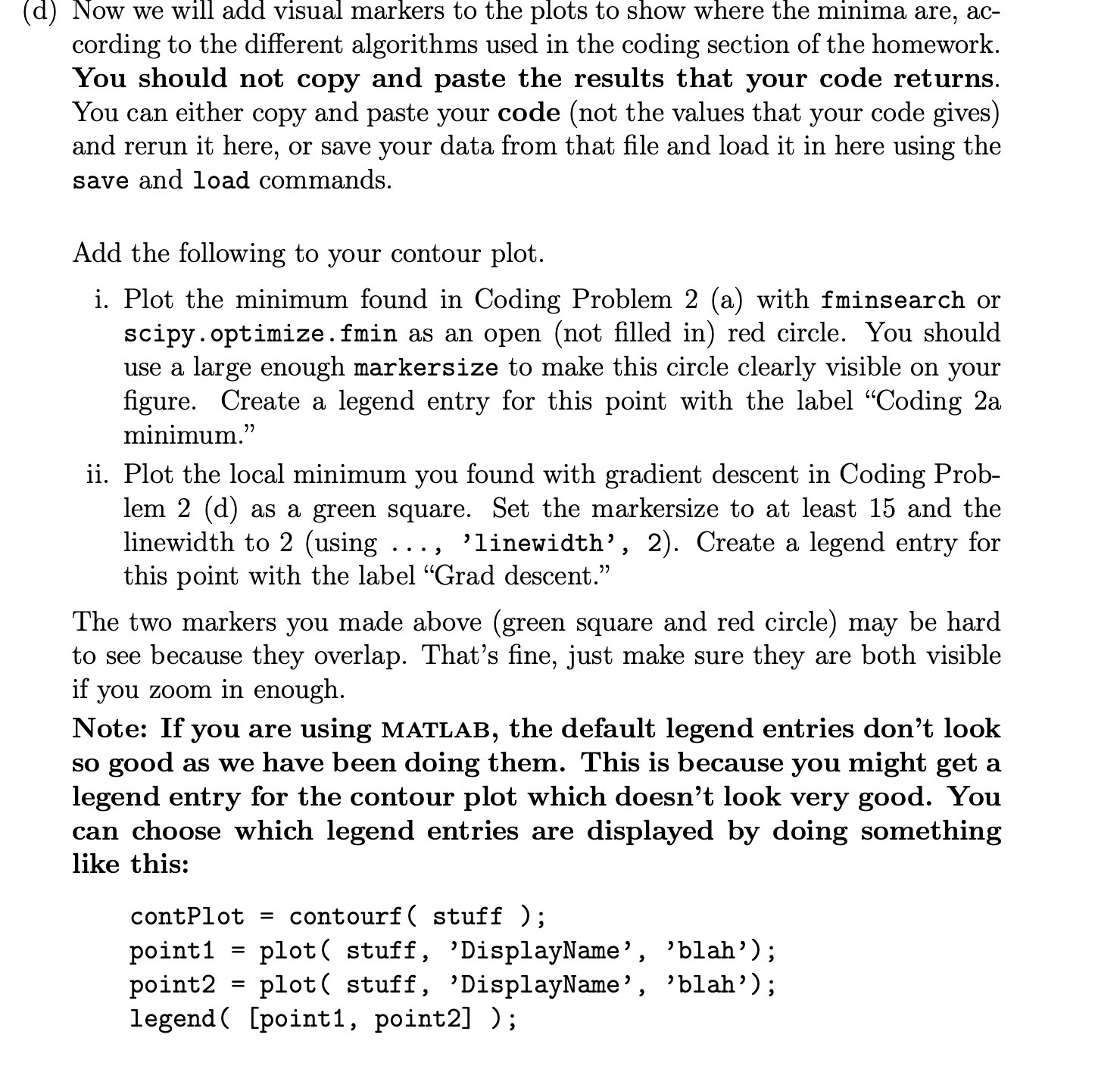
(d) Now we will add visual markers to the plots to show where the minima are, ac- cording to the different algorithms used in the coding section of the homework. You should not copy and paste the results that your code returns. You can either copy and paste your code (not the values that your code gives) and rerun it here, or save your data from that le and load it in here using the save and load commands. Add the following to your contour plot. i. Plot the minimum found in Coding Problem 2 (a) with fminsearch or scipy.optimize.fmin as an open (not lled in) red circle. You should use a large enough markersize to make this circle clearly Visible on your gure. Create a legend entry for this point with the label \"Coding 2a minimum.\" ii. Plot the local minimum you found with gradient descent in Coding Prob lem 2 (d) as a green square. Set the markersize to at least 15 and the linewidth to 2 (using . . . , 'linewidth' , 2). Create a legend entry for this point with the label \"Grad descent.\" The two markers you made above (green square and red circle) may be hard to see because they overlap. That's ne, just make sure they are both visible if you zoom in enough. Note: If you are using MATLAB, the default legend entries don't look so good as we have been doing them. This is because you might get a legend entry for the contour plot which doesn't look very good. You can choose which legend entries are displayed by doing something like this: contPlot - contourf( stuff ); point1 = plot( stuff, 'DisplayName', 'blah'); point2 = plot( stuff, 'DisplayName', 'blah'); legend( [point1, point2] )