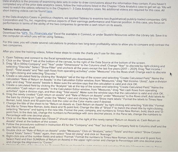
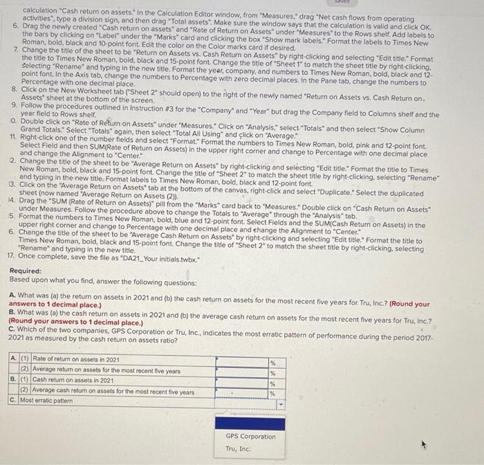
Data analytics is the process of examining data sets in order to draw conclusions about the information they contain. If you haven't completed any of the prior data analytics cases, follow the instructions listed in the Chapter 1 Data Analytics case to get set up. You will need to watch the videos referred to in the Chapters 1 - 3 Data Analytics cases. No additional videos are required for this case. All short training videos can be found here in the Data Analytics Cases in previous chapters, we applied Tableau to examine two (hypothetical) publicly traded companies: GPS Corporation and Tru, Inc. regarding various aspects of their earnings performance and financial position. In this case, you focus on performance in terms of the ability of the two companies to generate a cash return on its assets. Tableau Instructions: Download the "GPS Tru Financials.xlsx" Excel file available in Connect, or under Student Resources within the Library tab. Save it to the computer on which you will be using Tableau. For this case, you will create several calculations to produce two long-term profitability ratlos to allow you to compare and contrast the two companies After you view the training videos, follow these steps to create the charts you'll use for this case: 1. Open Tableau and connect to the Excel spreadsheet you downloaded 2. Click on the "Sheet t' tab at the bottom of the canvas, to the right of the Data Source at the bottom of the screen, 3. Drag "($ in 000s) Company" and "Year" under "Dimensions to the Columns shelf. Change "Year" to discrete by right-clicking and selecting "Discrete." Select "Show Filter" and uncheck all the years except the last five years (2017-2021). Drag "Net income/ (loss)'. "Total assets" and "Net cash flows from operating activities under "Measures into the Rows shell. Change each to discrete by right-clicking and selecting "Discrete." 4. Create a calculated field by clicking the "Analysis" tab at the top of the screen and selecting "Create Calculated field." Name the calculation "Rate of Return on Assets." In the Calculation Editor window, from "Measures," drag "Net Income /(loss)", type a division sign, and drag "Total assets" beside it . Make sure the window says that the calculation is valid and click OK. 5. Create a calculated field by clicking the "Analysis" tab at the top of the screen and selecting "Create Calculated field." Name the calculation "Cash return on assets. In the Calculation Editor window, from "Measures," drag "Net cash flows from operating activities", type a division sign, and then drag "Total assets". Make sure the window says that the calculation is valid and click OK. 6. Drag the newly created "Cosh return on assets" and "Rate of Return on Assets" under "Measures to the Rows shelf. Add labels to the bars by clicking on "Label" under the "Marks card and clicking the box "Show mark labels." Format the labels to Times New Roman, bold, black and 10-point font Edit the color on the Color marks card if desired. 7. Change the title of the sheet to be "Return on Assets vs. Cash Return on Assets" by right clicking and selecting "Edit title." Format the title to Times New Roman, bold, black and 15-point font Change the title of "Sheet 1" to match the sheet title by right-clicking, selecting "Rename" and typing in the new title Format the year, company, and numbers to Times New Roman, bold, black and 12. point font. In the Axis tab, change the numbers to Percentage with zero decimal places. In the Pane tab, change the numbers to Percentage with one decimal place. 8. Click on the New Worksheet tab (Sheet 2" should open) to the right of the newly named "Return on Assets vs. Cash Return on Assets" sheet at the bottom of the screen 9. Follow the procedures outlined in Instruction #3 for the "Company" and "Year" but drag the Company field to Columns shelf and the year field to Rows shelf. o. Double click on "Rate of Return on Assets" under "Measures." Click on "Analysis," select "Totals and then select "Show Column Grand Totals." Select "Totals" again, then select "Total All Using and click on "Average." 11. Right click one of the number fields and select "Format." Format the numbers to Times New Roman, bold, pink and 12 point font Select Field and then SUM(Rate of Return on Assets) in the upper right corner and change to Percentage with one decimal place and change the Alignment to "Center" - HAR calculation "Cash return on assets. In the Calculation Editor window, from "Measures." drag "Net cash flows from operating activities, type a division sign, and then drag "Total assets". Make sure the window says that the calculation is valid and click OK 6. Drag the newly created "Cash return on assets" and "Rate of Return on Assets" under "Measures to the Rows shelf. Add labels to the bars by clicking on "Label" under the "Marks" card and clicking the box "Show mark labels." Format the labels to Times New Roman, bold, black and 10-point font. Edit the color on the Color marks card if desired. 7. Change the title of the sheet to be "Return on Assets vs. Cash Return on Assets" by right-clicking and selecting "Edit title." Format the title to Times New Roman, bold, black and 15-point font Change the title of "Sheet 1" to match the sheet title by right-clicking, Selecting "Rename" and typing in the new title. Format the year, company, and numbers to Times New Roman, bold, black and 12- point font. In the Axis tab, change the numbers to Percentage with zero decimal places. In the Pane tab, change the numbers to Percentage with one decimal place. 8. Click on the New Worksheet tab (Sheet 2* should open) to the right of the newly named "Return on Assets vs. Cash Return on Assets sheet at the bottom of the screen, 9. Follow the procedures outlined in Instruction #3 for the "Company" and "Year" but drag the Company field to Columns shelf and the year field to Rows shelf o. Double click on "Rate of Return on Assets" under "Measures. Click on "Analysis," select "Totals" and then select "Show Column Grand Totals." Select "Totals" again, then select "Total All Using and click on "Average." 11. Right click one of the number fields and select "Format." Format the numbers to Times New Roman, bold, pink and 12-point font Select Field and then SUM(Rate of Return on Assets) in the upper right corner and change to Percentage with one decimal place and change the Alignment to "Center" 2. Change the title of the sheet to be "Average Return on Assets" by right-clicking and selecting "Edit title." Format the title to Times New Roman, bold, black and 15-point font. Change the title of "Sheet 2 to match the sheet title by right-clicking, selecting "Rename and typing in the new title. Format labels to Times New Roman, bold, black and 12-point font 13. Click on the "Average Return on Assets tab at the bottom of the canvas, right-click and select "Duplicate." Select the duplicated sheet (now named "Average Return on Assets (2)). 14. Drag the "SUM (Rate of Return on Assets) pill from the Marks" card back to "Measures." Double click on "Cash Return on Assets under Measures. Follow the procedure above to change the Totals to "Average through the "Analysis" tab. 5. Format the numbers to Times New Roman, bold, blue and 12-point font Select Fields and the SUM(Cash Return on Assets) in the upper right corner and change to Percentage with one decimal place and change the Alignment to "Center" 6. Change the title of the sheet to be "Average Cash Return on Assets" by right-clicking and selecting "Edit title." Format the title to Times New Roman, bold, black and 15-point font Change the title of "Sheet 2 to match the sheet title by right-clicking, selecting "Rename" and typing in the new title. 17. Once complete, save the file as "DA21_Your initials.twbx." Required: Based upon what you find answer the following questions: A. What was (a) the return on assets in 2021 and (b) the cash return on assets for the most recent five years Tru, Inc.? (Round your answers to 1 decimal place.) B. What was (a) the cash return on assets in 2021 and (b) the average cash return on assets for the most recent five years for Tru, Inc.? (Round your answers to 1 decimal place.) C. Which of the two companies, GPS Corporation or Tru, Inc., indicates the most erratic pattern of performance during the period 2017- 2021 as measured by the cash return on assets ratio? % A. (1) Rate of return on assets in 2021 (2) Average return on assets for the most recent five years B. (1) Cash return on assets in 2021 (2) Average cash return on assets for the most recent five years c. Most erratic pattern % % GPS Corporation Tru, Inc Data analytics is the process of examining data sets in order to draw conclusions about the information they contain. If you haven't completed any of the prior data analytics cases, follow the instructions listed in the Chapter 1 Data Analytics case to get set up. You will need to watch the videos referred to in the Chapters 1 - 3 Data Analytics cases. No additional videos are required for this case. All short training videos can be found here in the Data Analytics Cases in previous chapters, we applied Tableau to examine two (hypothetical) publicly traded companies: GPS Corporation and Tru, Inc. regarding various aspects of their earnings performance and financial position. In this case, you focus on performance in terms of the ability of the two companies to generate a cash return on its assets. Tableau Instructions: Download the "GPS Tru Financials.xlsx" Excel file available in Connect, or under Student Resources within the Library tab. Save it to the computer on which you will be using Tableau. For this case, you will create several calculations to produce two long-term profitability ratlos to allow you to compare and contrast the two companies After you view the training videos, follow these steps to create the charts you'll use for this case: 1. Open Tableau and connect to the Excel spreadsheet you downloaded 2. Click on the "Sheet t' tab at the bottom of the canvas, to the right of the Data Source at the bottom of the screen, 3. Drag "($ in 000s) Company" and "Year" under "Dimensions to the Columns shelf. Change "Year" to discrete by right-clicking and selecting "Discrete." Select "Show Filter" and uncheck all the years except the last five years (2017-2021). Drag "Net income/ (loss)'. "Total assets" and "Net cash flows from operating activities under "Measures into the Rows shell. Change each to discrete by right-clicking and selecting "Discrete." 4. Create a calculated field by clicking the "Analysis" tab at the top of the screen and selecting "Create Calculated field." Name the calculation "Rate of Return on Assets." In the Calculation Editor window, from "Measures," drag "Net Income /(loss)", type a division sign, and drag "Total assets" beside it . Make sure the window says that the calculation is valid and click OK. 5. Create a calculated field by clicking the "Analysis" tab at the top of the screen and selecting "Create Calculated field." Name the calculation "Cash return on assets. In the Calculation Editor window, from "Measures," drag "Net cash flows from operating activities", type a division sign, and then drag "Total assets". Make sure the window says that the calculation is valid and click OK. 6. Drag the newly created "Cosh return on assets" and "Rate of Return on Assets" under "Measures to the Rows shelf. Add labels to the bars by clicking on "Label" under the "Marks card and clicking the box "Show mark labels." Format the labels to Times New Roman, bold, black and 10-point font Edit the color on the Color marks card if desired. 7. Change the title of the sheet to be "Return on Assets vs. Cash Return on Assets" by right clicking and selecting "Edit title." Format the title to Times New Roman, bold, black and 15-point font Change the title of "Sheet 1" to match the sheet title by right-clicking, selecting "Rename" and typing in the new title Format the year, company, and numbers to Times New Roman, bold, black and 12. point font. In the Axis tab, change the numbers to Percentage with zero decimal places. In the Pane tab, change the numbers to Percentage with one decimal place. 8. Click on the New Worksheet tab (Sheet 2" should open) to the right of the newly named "Return on Assets vs. Cash Return on Assets" sheet at the bottom of the screen 9. Follow the procedures outlined in Instruction #3 for the "Company" and "Year" but drag the Company field to Columns shelf and the year field to Rows shelf. o. Double click on "Rate of Return on Assets" under "Measures." Click on "Analysis," select "Totals and then select "Show Column Grand Totals." Select "Totals" again, then select "Total All Using and click on "Average." 11. Right click one of the number fields and select "Format." Format the numbers to Times New Roman, bold, pink and 12 point font Select Field and then SUM(Rate of Return on Assets) in the upper right corner and change to Percentage with one decimal place and change the Alignment to "Center" - HAR calculation "Cash return on assets. In the Calculation Editor window, from "Measures." drag "Net cash flows from operating activities, type a division sign, and then drag "Total assets". Make sure the window says that the calculation is valid and click OK 6. Drag the newly created "Cash return on assets" and "Rate of Return on Assets" under "Measures to the Rows shelf. Add labels to the bars by clicking on "Label" under the "Marks" card and clicking the box "Show mark labels." Format the labels to Times New Roman, bold, black and 10-point font. Edit the color on the Color marks card if desired. 7. Change the title of the sheet to be "Return on Assets vs. Cash Return on Assets" by right-clicking and selecting "Edit title." Format the title to Times New Roman, bold, black and 15-point font Change the title of "Sheet 1" to match the sheet title by right-clicking, Selecting "Rename" and typing in the new title. Format the year, company, and numbers to Times New Roman, bold, black and 12- point font. In the Axis tab, change the numbers to Percentage with zero decimal places. In the Pane tab, change the numbers to Percentage with one decimal place. 8. Click on the New Worksheet tab (Sheet 2* should open) to the right of the newly named "Return on Assets vs. Cash Return on Assets sheet at the bottom of the screen, 9. Follow the procedures outlined in Instruction #3 for the "Company" and "Year" but drag the Company field to Columns shelf and the year field to Rows shelf o. Double click on "Rate of Return on Assets" under "Measures. Click on "Analysis," select "Totals" and then select "Show Column Grand Totals." Select "Totals" again, then select "Total All Using and click on "Average." 11. Right click one of the number fields and select "Format." Format the numbers to Times New Roman, bold, pink and 12-point font Select Field and then SUM(Rate of Return on Assets) in the upper right corner and change to Percentage with one decimal place and change the Alignment to "Center" 2. Change the title of the sheet to be "Average Return on Assets" by right-clicking and selecting "Edit title." Format the title to Times New Roman, bold, black and 15-point font. Change the title of "Sheet 2 to match the sheet title by right-clicking, selecting "Rename and typing in the new title. Format labels to Times New Roman, bold, black and 12-point font 13. Click on the "Average Return on Assets tab at the bottom of the canvas, right-click and select "Duplicate." Select the duplicated sheet (now named "Average Return on Assets (2)). 14. Drag the "SUM (Rate of Return on Assets) pill from the Marks" card back to "Measures." Double click on "Cash Return on Assets under Measures. Follow the procedure above to change the Totals to "Average through the "Analysis" tab. 5. Format the numbers to Times New Roman, bold, blue and 12-point font Select Fields and the SUM(Cash Return on Assets) in the upper right corner and change to Percentage with one decimal place and change the Alignment to "Center" 6. Change the title of the sheet to be "Average Cash Return on Assets" by right-clicking and selecting "Edit title." Format the title to Times New Roman, bold, black and 15-point font Change the title of "Sheet 2 to match the sheet title by right-clicking, selecting "Rename" and typing in the new title. 17. Once complete, save the file as "DA21_Your initials.twbx." Required: Based upon what you find answer the following questions: A. What was (a) the return on assets in 2021 and (b) the cash return on assets for the most recent five years Tru, Inc.? (Round your answers to 1 decimal place.) B. What was (a) the cash return on assets in 2021 and (b) the average cash return on assets for the most recent five years for Tru, Inc.? (Round your answers to 1 decimal place.) C. Which of the two companies, GPS Corporation or Tru, Inc., indicates the most erratic pattern of performance during the period 2017- 2021 as measured by the cash return on assets ratio? % A. (1) Rate of return on assets in 2021 (2) Average return on assets for the most recent five years B. (1) Cash return on assets in 2021 (2) Average cash return on assets for the most recent five years c. Most erratic pattern % % GPS Corporation Tru, Inc