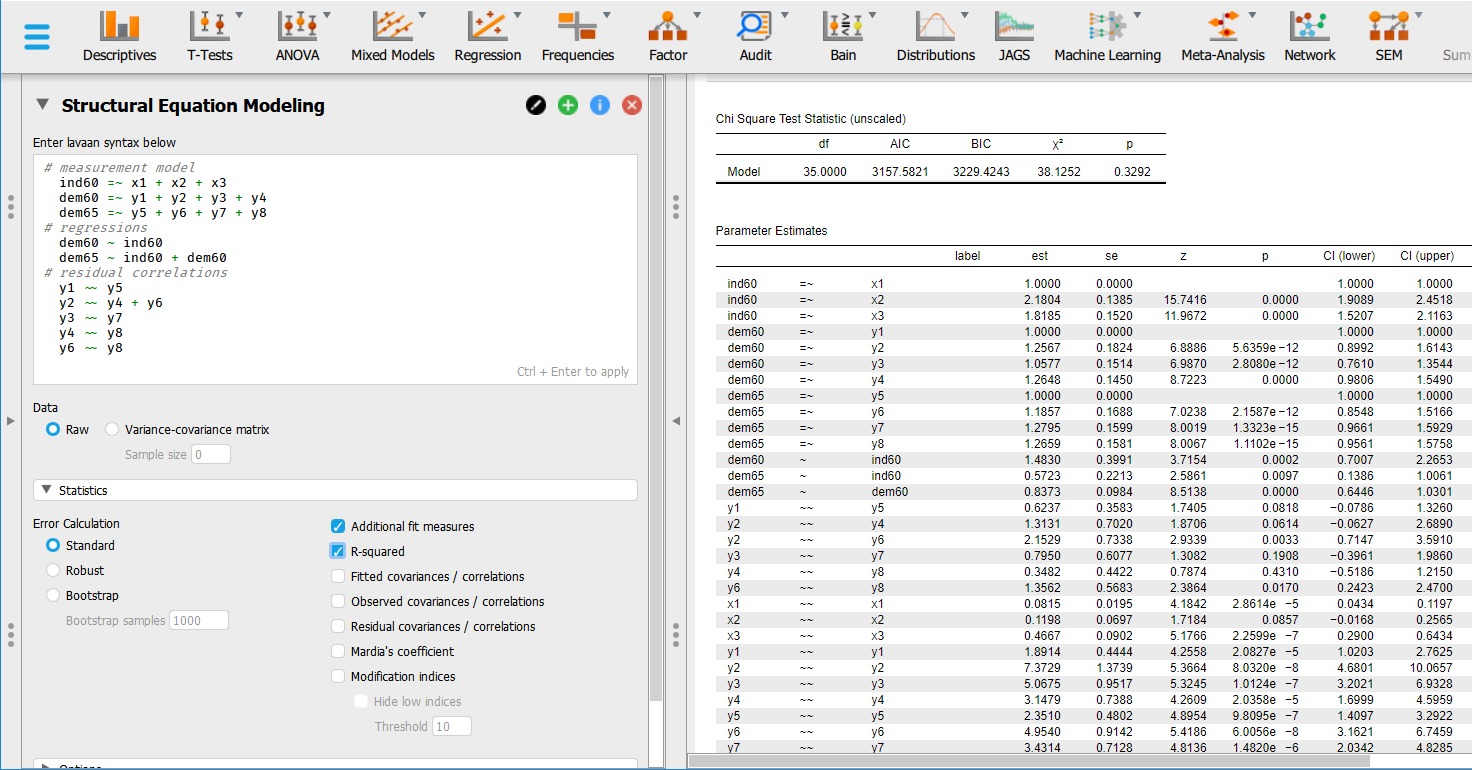
Descriptives T-Tests ANOVA Mixed Models Regression Frequencies Factor Audit Bain Distributions JAGS Machine Learning Meta-Analysis Network SEM Sum V Structural Equation Modeling +i x Chi Square Test Statistic (unscaled) Enter lavaan syntax below di AIC BIC # measurement model Model 35.0000 3157.5821 3229.4243 38. 1252 0.3292 ind60 =~ x1 + x2 + x3 dem60 =~ yl + y2 + y3 + y4 dem65 =~ y5 + y6 + y7 + y8 # regressions Parameter Estimates dem60 ~ ind60 labe est Se Z p CI (lower) CI (upper) dem65 ~ ind60 + dem60 # residual correlations ind60 1.0000 0.0000 1.0000 1.0000 yl ~ y5 x1 ind60 x2 2.1804 0. 1385 15.7416 0.0000 1.9089 2.4518 y2 ~ y4 + y6 y3 ind60 x3 1.8185 0. 1520 11.9672 0.0000 1.5207 2.1163 y4 dem60 y1 1.0000 0.0000 1.0000 1.0000 y6- V8 dem60 y2 1.2567 0.1824 6.8886 5.6359e -12 0.8992 1.6143 dem60 y3 1.0577 0. 1514 6.9870 2.8080e -12 0.7610 1.3544 Ctrl + Enter to apply dem60 y4 1.2648 0.1450 8.7223 0.0000 0.9806 1.5490 dem65 y5 1.0000 0.0000 1.0000 1.0000 Data dem65 y6 1.1857 0. 1688 7.0238 2.1587e -12 0.8548 1.5166 0.9661 1.5929 O Raw O Variance-covariance matrix dem65 y7 1.2795 0. 1599 8.0019 1.3323e -15 dem65 V8 1.2659 0. 1581 8.0067 1.1102e -15 0.9561 1.5758 Sample size |0 dem60 ind60 1.4830 0.3991 3.7154 0.0002 0.7007 2.2653 dem65 ind60 0.5723 0.2213 2.5861 0.0097 0. 1386 1.0061 Statistics dem65 dem60 0.8373 0.0984 8.5138 0.0000 0.6446 1.0301 y1 y5 0.6237 0.3583 1.7405 0.0818 -0.0786 1.3260 Error Calculation Additional fit measures y2 y4 1.3131 0.7020 1.8706 0.0614 -0.0627 2.6890 y2 y6 2.1529 0.7338 2.9339 0.0033 0.7147 3.5910 O Standard R-squared y7 0.7950 0.6077 1.3082 0. 1908 -0.3961 1.9860 Robust y4 y8 0.3482 0.4422 0.7874 0.4310 -0.5186 1.2150 Fitted covariances / correlations y6 y8 1.3562 0.5683 2.3864 0.0170 0.2423 2.4700 Bootstrap O Observed covariances / correlations x1 x1 0.0815 0.0195 4.1842 2.8614e -5 0.0434 0. 1197 0.0857 -0.0168 0.2565 Bootstrap samples 1000 x2 X2 0. 1198 0.0697 1.7184 Residual covariances / correlations x3 x3 0.4667 0.0902 5.1766 2.2599e -7 0.2900 0.6434 Mardia's coefficient 1.8914 0.4444 4.2558 2.0827e -5 1.0203 2.7625 y2 y2 7.3729 1.3739 5.3664 8.0320e -8 4.6801 10.0657 Modification indices y3 5.0675 0.9517 5.3245 1.0124e -7 3.2021 6.9328 Hide low indices y4 3.1479 0.7388 4.2609 2.0358e -5 1.6999 4.5959 NOGEO y5 2.3510 0.4802 4.8954 9.8095e -7 1.4097 3.2922 Threshold 10 y6 4.9540 0.9142 5.4186 6.0056e -8 3.1621 6.7459 y7 3.4314 0.7128 4.8136 1.4820e -6 2.0342 4.8285