Differential Equations MATLAB Project: Relating ODE Equations to Real-Life Situations

Please convert these procedure into MATLAB codes : Population Growth

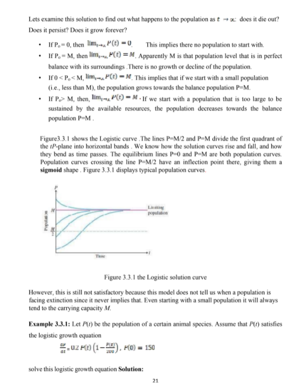
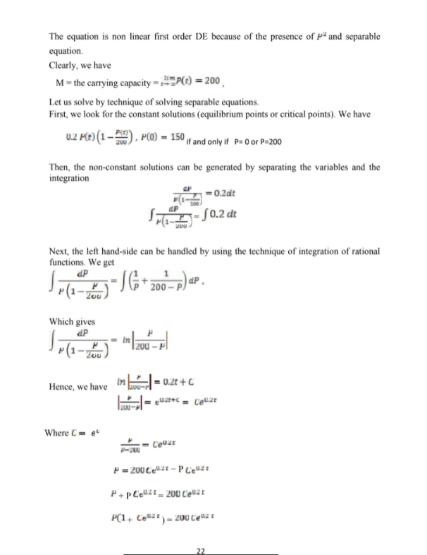
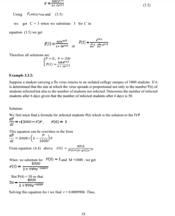
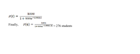
3.3 Population Growth In order to illustrate the use of differential equations with regard to population problems we consider the easiest mathematical model offered to govern the population dynamics of a certain species. One of the earliest attempts to model human population growth by means of mathematics was by the English economist Thomas Malthus in 1798. Essentially, the idea of the Malthusian model is the assumption that the rate at which a population of a country grows at a certain time is proportional to the total population of the country at that time . In mathematical terms, if P(t) denotes the total population at time t, then this assumption can be expressed as dP DAP(!) (3.1) dt where k is called the growth constant or the decay constant, as appropriate. Solution of equation (4.1) will provide population at any future time t. This simple model which does not take many factors into account (immigration and emigration, for example) that can influence human populations to either grow or decline, nevertheless turned out to be fairly accurate in predicting the population. dP(t) The differential equation O kP(() , where P(t) denotes population at time t and k is a di constant of proportionality, serves as a model for population growth and decay of insects, animals and human population at certain places and duration. It is fairly easy to see that if k > 0, we have growth, and if k 0, then the population grows and continues to expand to infinity, that is, lim P(t) = w t w . if M, then, lim,-. P() = M . If we start with a population that is too large to be sustained by the available resources, the population decreases towards the balance population P=M . Figure3.3.1 shows the Logistic curve . The lines P-M/2 and P-M divide the first quadrant of the P-plane into horizontal bands . We know how the solution curves rise and fall, and how they bend as time passes. The equilibrium lines P=0 and P=M are both population curves. Population curves crossing the line P=M/2 have an inflection point there, giving them a sigmoid shape . Figure 3.3.1 displays typical population curves. population Populari an Thin Figure 3.3.1 the Logistic solution curve However, this is still not satisfactory because this model does not tell us when a population is facing extinction since it never implies that. Even starting with a small population it will always tend to the carrying capacity M. Example 3.3.1: Let P() be the population of a certain animal species. Assume that P() satisfies the logistic growth equation "- 0.2 P(() (1-2), P(0) = 150 solve this logistic growth equation Solution:The equation is non linear first order DE because of the presence of - and separable equation. Clearly, we have M - the carrying capacity = - HimP(t) = 200 Let us solve by technique of solving separable equations. First, we look for the constant solutions (equilibrium points or critical points). We have 0.2 P(t) (1 -=) . P(0) = 150 if and only if P= 0 or P=200 Then, the non-constant solutions can be generated by separating the variables and the integration = 0.2dt ap S0.2 dt Next, the left hand-side can be handled by using the technique of integration of rational functions. We get dP JC+ 1 200 - p) ap . Which gives dP In 200 -F Zou Hence, we have In Toy = 0.21 + C Where C - POT = COUZE = 200CZE -PCuz: P+PC-UZE_ 200 Cour P(1 + Cell) = 200Cel1+ Ceout (3.5) Using P.=plol =1au and (3.5) we get C = 3 when we substitute 3 for C in equation (3.5) we get PO)= 1+ 14731 or Therefore all solutions are (P =0, P= 200 P(D) = Example 3.3.2: Suppose a student carrying a flu virus returns to an isolated college campus of 1000 students. If it is determined that the rate at which the virus spreads is proportional not only to the number P(t) of students infected but also to the number of students not infected. Determine the number of infected students after 6 days given that the number of infected students after 4 days is 50. Solution. We first must find a formula for infected students P(t) which is the solution to the IVP dP dt - =(1000-P)P . H(0) = 1 This equation can be rewritten in the form dP = 1000 r (1 - P 1000 MPLO From equation (4.4) above P(t) = p(Q)+ (M-p(0))- When we substitute for (0) - 1and M=1000, we get 1000 P(t) = 1+yyye 10uurt But P(4) = 50 so that 1000 50 - 1+999e-40WP Solving this equation for r we find r = 0.0009906: Thus, 231000 P() = Finally, P(6) = Itmay-tew ( = 276 students