Discuss your key findings:

1. Did dimensionality reduction improve performance or interpretation?
2. Which classifier performed best and why?
3. What did the clusters reveal about your data?
4. Were there any surprises or inconsistencies in the results?

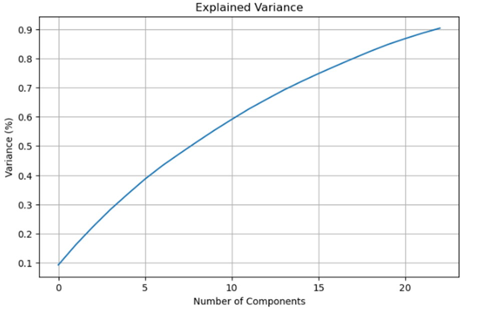
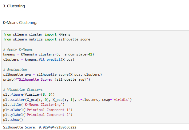
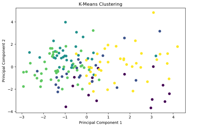
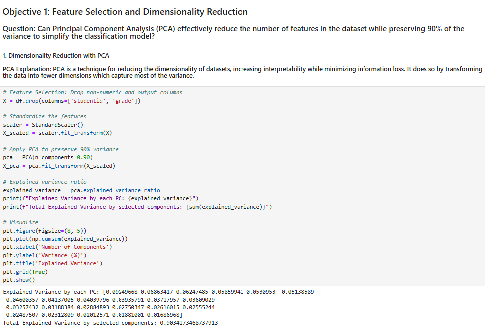
Objective 1: Feature Selection and Dimensionality Reduction Question: Can Principal Component Analysis (PCA) effectively reduce the number of features in the dataset while preserving 90% of the variance to simplify the classification model? 1. Dimensionality Reduction with PCA PCA Explanation: PCA is a technique for reducing the dimensionality of datasets, increasing interpretability while minimizing information loss. It does so by transforming the data into fewer dimensions which capture most of the variance. # Feature Selection: Drop non-numeric and output columns X = df . drop(columns=[ 'studentid' , 'grade' ]) # Standardize the features scaler = StandardScaler() X_scaled = scaler. fit_transform(X) # Apply PCA to preserve 90% variance pca = PCA(n_components=0.90) X_pca = pca. fit_transform(X_scaled) # Explained variance ratio explained_variance = pca . explained_variance_ratio_ print (f"Explained Variance by each PC: {explained_variance}") print (f"Total Explained Variance by selected components: {sum(explained_variance)}") # Visualize pit. figure(figsize=(8, 5)) pit. plot (np. cumsum(explained_variance) ) pit. xlabel('Number of Components' ) pit. ylabel('Variance (*) ' ) pit. title('Explained Variance' ) pit. grid(True) pit . show( ) Explained Variance by each PC: [0. 09249668 0. 06863417 0. 06247485 0. 05859941 0.0530953 0.05138589 0. 04600357 0. 04137005 0.04039796 0. 03935791 0.03717957 0.03609029 0.03257432 0.03188384 0.02884893 0.02750347 0.02616015 0.02555244 0. 02487507 0. 02312809 0.02012571 0. 01881091 0.01686968] Total Explained Variance by selected components: 0.9034173468737913\f3. Clustering K-Means Clustering: from sklearn . cluster import KMeans from sklearn. metrics import silhouette_score # Apply K-Means kmeans = KMeans (n_clusters=5, random_state=42) clusters = kmeans . fit_predict(X_pca) # Evaluation silhouette_avg = silhouette_score(X_pca, clusters) print (f"Silhouette Score: {silhouette_avg}") # Visualize Clusters pit. figure(figsize=(8, 5)) pit. scatter (X_pca[:, 0], X_pca[:, 1], c=clusters, cmap='viridis') plt . title('K-Means Clustering" ) pit. xlabel('Principal Component 1" ) pit. ylabel('Principal Component 2' ) pit . show() Silhouette Score: 0.02940472180636222\f