

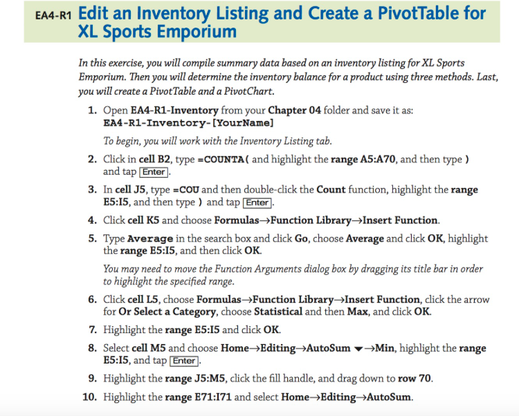
Question: EA4-R1 Edit an Inventory Listing and Create a PivotTable for XL Sports Emporium In this exercise, you will compile summary data based on an inventory
![folder and save it as: EA4-R1-Inventory-[YourName] 2. Click in cell B2, type](https://dsd5zvtm8ll6.cloudfront.net/si.experts.images/questions/2024/09/66f0f7e628289_13366f0f7e596f21.jpg)

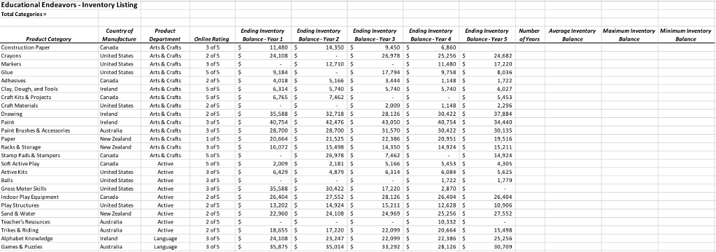
EA4-R1 Edit an Inventory Listing and Create a PivotTable for XL Sports Emporium In this exercise, you will compile summary data based on an inventory listing for XL Sports Emporium. Then you will determine the inventory balance for a product using three methods. Last, you will create a PivotTable and a PivotChart. 1. Open EA4-R1-Inventory from your Chapter 04 folder and save it as: EA4-R1-Inventory-[YourName] 2. Click in cell B2, type COUNTA ( and highlight the range A5:A70, and then type ) 3. In cell J5, type cOU and then double-click the Count function, highlight the range 4. Click cell K5 and choose FormulasFunction LibraryInsert Function. 5. Type Average in the search box and click Go, choose Average and click OK, highlight To begin, you will work with the Inventory Listing tab and tap [Enter ES:I5, and then type) and tap Enter the range E5:I5, and then click OK. You may need to move the Function Arguments dialog box by dragging its title bar in order to highlight the specified range Click cell L5, choose Formulas Function LibraryInsert Function, click the arrow for Or Select a Category, choose Statistical and then Max, and click OK. 6. 7. Highlight the range E5:I5 and cdlick OK. 8, Select cell M5 and choose HomeEditingAutoSum Min, highlight the range E5:15, and tap Enter 9. Highlight the range J5:M5, click the fill handle, and drag down to row 70 10. Highlight the range E71:171 and select Home>Editing ->AutoSum. EA4-R1 Edit an Inventory Listing and Create a PivotTable for XL Sports Emporium In this exercise, you will compile summary data based on an inventory listing for XL Sports Emporium. Then you will determine the inventory balance for a product using three methods. Last, you will create a PivotTable and a PivotChart. 1. Open EA4-R1-Inventory from your Chapter 04 folder and save it as: EA4-R1-Inventory-[YourName] 2. Click in cell B2, type COUNTA ( and highlight the range A5:A70, and then type ) 3. In cell J5, type cOU and then double-click the Count function, highlight the range 4. Click cell K5 and choose FormulasFunction LibraryInsert Function. 5. Type Average in the search box and click Go, choose Average and click OK, highlight To begin, you will work with the Inventory Listing tab and tap [Enter ES:I5, and then type) and tap Enter the range E5:I5, and then click OK. You may need to move the Function Arguments dialog box by dragging its title bar in order to highlight the specified range Click cell L5, choose Formulas Function LibraryInsert Function, click the arrow for Or Select a Category, choose Statistical and then Max, and click OK. 6. 7. Highlight the range E5:I5 and cdlick OK. 8, Select cell M5 and choose HomeEditingAutoSum Min, highlight the range E5:15, and tap Enter 9. Highlight the range J5:M5, click the fill handle, and drag down to row 70 10. Highlight the range E71:171 and select Home>Editing ->AutoSum
Step by Step Solution
There are 3 Steps involved in it

Get step-by-step solutions from verified subject matter experts