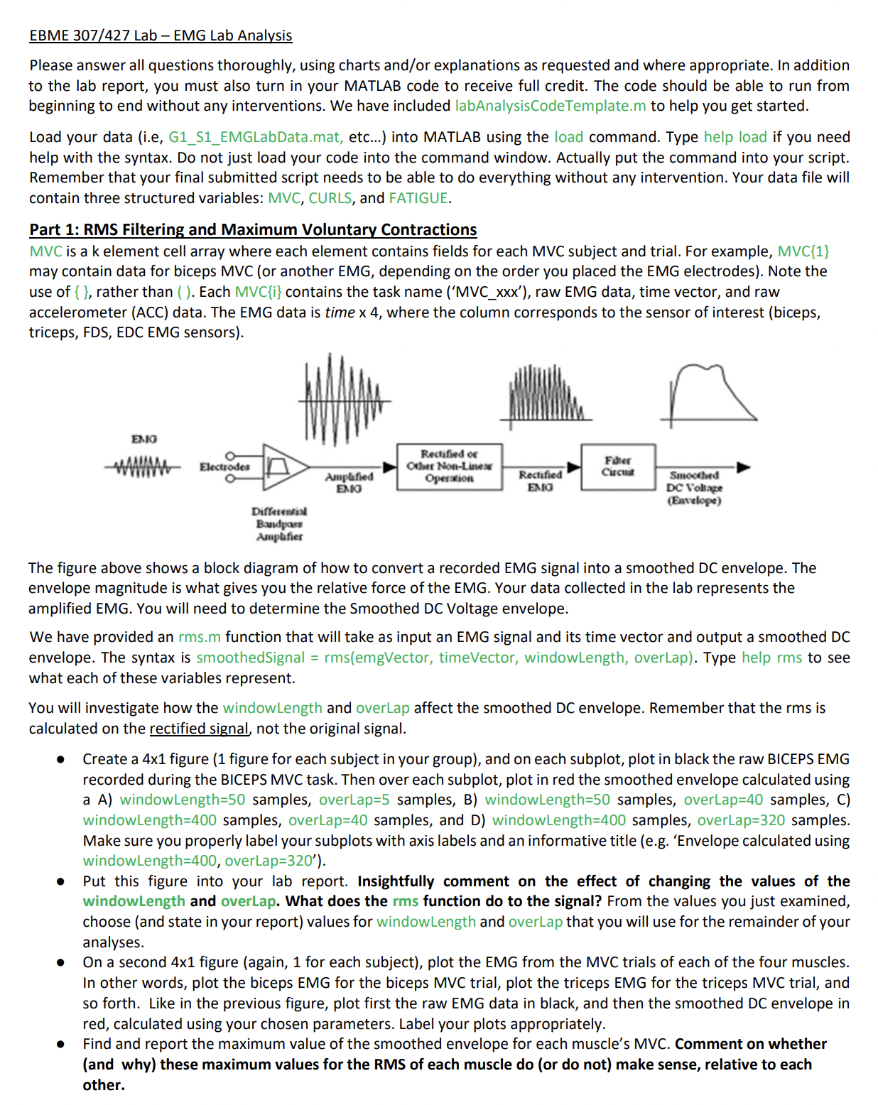
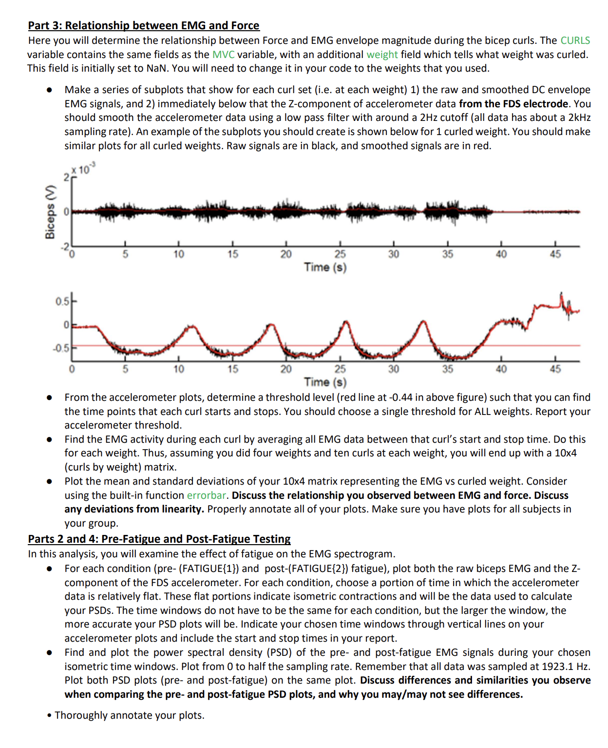
EBME 307/427 Lab EMG Lab Analysis Please answer all questions thoroughly, using charts and/or explanations as requested and where appropriate. In addition to the lab report, you must also turn in your MATLAB code to receive full credit. The code should be able to run from beginning to end without any interventions. We have included labAnalysisCodeTemplate.m to help you get started. Load your data (i.e, G1_S1_EMGLabData.mat, etc...) into MATLAB using the load command. Type help load if you need help with the syntax. Do not just load your code into the command window. Actually put the command into your script. Remember that your final submitted script needs to be able to do everything without any intervention. Your data file will contain three structured variables: MVC, CURLS, and FATIGUE. Part 1. RMS Filtering and Maximum Voluntary Contractions MVC is a k element cell array where each element contains fields for each MVC subject and trial. For example, MVC{1} may contain data for biceps MVC (or another EMG, depending on the order you placed the EMG electrodes). Note the use of { }, rather than ( ). Each MVC{i} contains the task name ('MVC_xxx'), raw EMG data, time vector, and raw accelerometer (ACC) data. The EMG data is time x 4, where the column corresponds to the sensor of interest (biceps, triceps, FDS, EDC EMG sensors). EMG FM EMO Dn m\\aap (Eavelope) Dafferentsnd Bwndpass Asmplfier The figure above shows a block diagram of how to convert a recorded EMG signal into a smoothed DC envelope. The envelope magnitude is what gives you the relative force of the EMG. Your data collected in the lab represents the amplified EMG. You will need to determine the Smoothed DC Voltage envelope. We have provided an rms.m function that will take as input an EMG signal and its time vector and output a smoothed DC envelope. The syntax is smoothedSignal = rms(emgVector, timeVector, windowlLength, overLap). Type help rms to see what each of these variables represent. You will investigate how the windowlLength and overlLap affect the smoothed DC envelope. Remember that the rms is calculated on the rectified signal, not the original signal. e Create a 4x1 figure (1 figure for each subject in your group), and on each subplot, plotin black the raw BICEPS EMG recorded during the BICEPS MVC task. Then over each subplot, plot in red the smoothed envelope calculated using a A) windowlength=50 samples, overLap=5 samples, B) windowlLength=50 samples, overLap=40 samples, C) windowLength=400 samples, overLap=40 samples, and D) windowLength=400 samples, overLap=320 samples. Make sure you properly label your subplots with axis labels and an informative title (e.g. 'Envelope calculated using windowLength=400, overLap=320'). e Put this figure into your lab report. Insightfully comment on the effect of changing the values of the windowlLength and overLap. What does the rms function do to the signal? From the values you just examined, choose (and state in your report) values for windowlength and overLap that you will use for the remainder of your analyses. e On asecond 4x1 figure (again, 1 for each subject), plot the EMG from the MVC trials of each of the four muscles. In other words, plot the biceps EMG for the biceps MVC trial, plot the triceps EMG for the triceps MVC trial, and so forth. Like in the previous figure, plot first the raw EMG data in black, and then the smoothed DC envelope in red, calculated using your chosen parameters. Label your plots appropriately. e Find and report the maximum value of the smoothed envelope for each muscle's MVC. Comment on whether (and why) these maximum values for the RMS of each muscle do (or do not) make sense, relative to each other. Part 3: Relationship between EMG and Force Here you will determine the relationship between Force and EMG envelope magnitude during the bicep curls. The CURLS variable contains the same fields as the \\MVC variable, with an additional weight field which tells what weight was curled. This field is initially set to NaN. You will need to change it in your code to the weights that you used. e Make a series of subplots that show for each curl set (i.e. at each weight) 1) the raw and smoothed DC envelope EMG signals, and 2) immediately below that the Z-component of accelerometer data from the FDS electrode. You should smooth the accelerometer data using a low pass filter with around a 2Hz cutoff (all data has about a 2kHz sampling rate). An example of the subplots you should create is shown below for 1 curled weight. You should make similar plots for all curled weights. Raw signals are in black, and smoothed signals are in red. x10" 2 a0 2 m %o 5 10 15 20 25 30 35 40 45 Time (s) 05 0 05 0 5 10 15 20 25 30 35 40 45 Time (s) e From the accelerometer plots, determine a threshold level (red line at -0.44 in above figure) such that you can find the time points that each curl starts and stops. You should choose a single threshold for ALL weights. Report your accelerometer threshold. e Find the EMG activity during each curl by averaging all EMG data between that curl's start and stop time. Do this for each weight. Thus, assuming you did four weights and ten curls at each weight, you will end up with a 10x4 (curls by weight) matrix. e Plot the mean and standard deviations of your 10x4 matrix representing the EMG vs curled weight. Consider using the built-in function errorbar. Discuss the relationship you observed between EMG and force. Discuss any deviations from linearity. Properly annotate all of your plots. Make sure you have plots for all subjects in your group. Parts 2 and 4: Pre-Fatigue and Post-Fatigue Testing In this analysis, you will examine the effect of fatigue on the EMG spectrogram. For each condition (pre- (FATIGUE{1}) and post-(FATIGUE{2}) fatigue), plot both the raw biceps EMG and the Z- component of the FDS accelerometer. For each condition, choose a portion of time in which the accelerometer data is relatively flat. These flat portions indicate isometric contractions and will be the data used to calculate your PSDs. The time windows do not have to be the same for each condition, but the larger the window, the more accurate your PSD plots will be. Indicate your chosen time windows through vertical lines on your accelerometer plots and include the start and stop times in your report. Find and plot the power spectral density (PSD) of the pre- and post-fatigue EMG signals during your chosen isometric time windows. Plot from 0 to half the sampling rate. Remember that all data was sampled at 1923.1 Hz. Plot both PSD plots (pre- and post-fatigue) on the same plot. Discuss differences and similarities you observe when comparing the pre- and post-fatigue PSD plots, and why you may/may not see differences. * Thoroughly annotate your plots