

Enterprise Industries produces Fresh, a brand of liquid laundry detergent. In order to manage its inventory...
Fantastic news! We've Found the answer you've been seeking!
Question:


Transcribed Image Text:
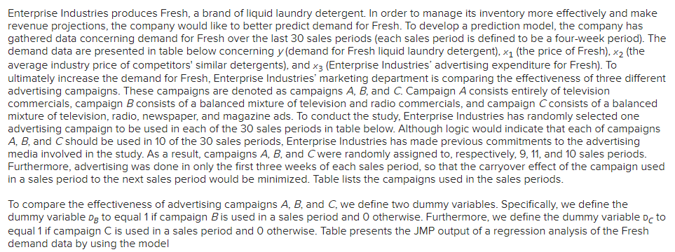
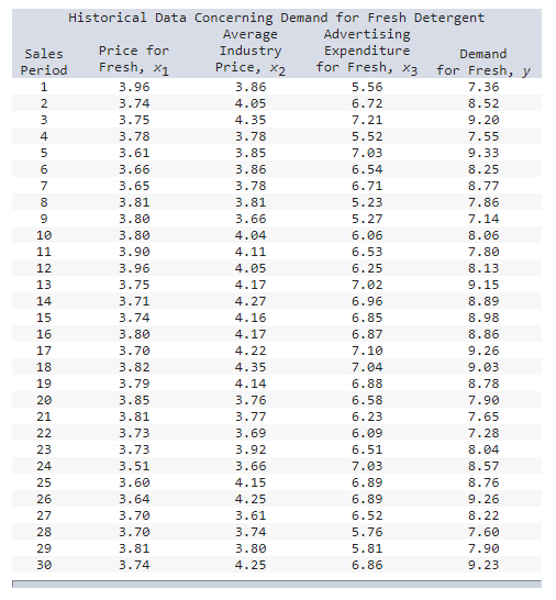
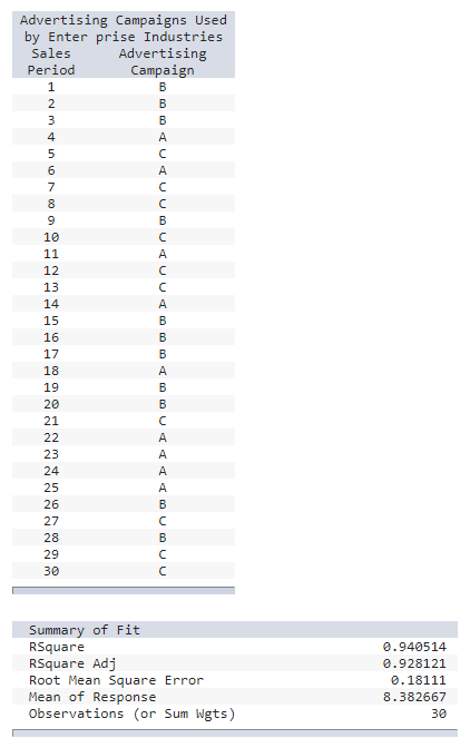
Enterprise Industries produces Fresh, a brand of liquid laundry detergent. In order to manage its inventory more effectively and make revenue projections, the company would like to better predict demand for Fresh. To develop a prediction model, the company has gathered data concerning demand for Fresh over the last 30 sales periods (each sales period is defined to be a four-week period). The demand data are presented in table below concerning y (demand for Fresh liquid laundry detergent), x1 (the price of Fresh), x2 (the average industry price of competitors' similar detergents), and x3 (Enterprise Industries' advertising expenditure for Fresh). To ultimately increase the demand for Fresh, Enterprise Industries' marketing department is comparing the effectiveness of three different advertising campaigns. These campaigns are denoted as campaigns A, B, and C. Campaign A consists entirely of television commercials, campaign B consists of a balanced mixture of television and radio commercials, and campaign C consists of a balanced mixture of television, radio, newspaper, and magazine ads. To conduct the study, Enterprise Industries has randomly selected one advertising campaign to be used in each of the 30 sales periods in table below. Although logic would indicate that each of campaigns A, B, and C should be used in 10 of the 30 sales periods, Enterprise Industries has made previous commitments to the advertising media involved in the study. As a result, campaigns A, B, and C were randomly assigned to, respectively, 9, 11, and 10 sales periods. Furthermore, advertising was done in only the first three weeks of each sales period, so that the carryover effect of the campaign used in a sales period to the next sales period would be minimized. Table lists the campaigns used in the sales periods. To compare the effectiveness of advertising campaigns A, B, and C, we define two dummy variables. Specifically, we define the dummy variable Dg to equal 1 if campaign B is used in a sales period and 0 otherwise. Furthermore, we define the dummy variable DC to equal 1 if campaign C is used in a sales period and 0 otherwise. Table presents the JMP output of a regression analysis of the Fresh demand data by using the model Historical Data Concerning Demand for Fresh Detergent Average Advertising Sales Price for Industry Expenditure Demand Period Fresh, x1 Price, x2 for Fresh, x3 for Fresh, y 1234562345678902234IONWOO 3.96 3.86 5.56 7.36 3.74 4.05 6.72 8.52 3.75 4.35 7.21 9.20 3.78 3.78 5.52 7.55 3.61 3.85 7.03 9.33 3.66 3.86 6.54 8.25 3.65 3.78 6.71 8.77 3.81 3.81 5.23 7.86 3.80 3.66 5.27 7.14 3.80 4.04 6.06 8.06 11 3.90 4.11 6.53 7.80 3.96 4.05 6.25 8.13 3.75 4.17 7.02 9.15 3.71 4.27 6.96 8.89 3.74 4.16 6.85 8.98 3.80 4.17 6.87 8.86 3.70 4.22 7.10 9.26 3.82 4.35 7.04 9.03 3.79 4.14 6.88 8.78 3.85 3.76 6.58 7.90 3.81 3.77 6.23 7.65 3.73 3.69 6.09 7.28 3.73 3.92 6.51 8.04 3.51 3.66 7.03 8.57 3.60 4.15 6.89 8.76 3.64 4.25 6.89 9.26 3.70 3.61 6.52 8.22 3.70 3.74 5.76 7.60 3.81 3.80 5.81 7.90 3.74 4.25 6.86 9.23 Advertising Campaigns Used by Enter prise Industries Sales Period 1 Advertising Campaign B 14 12345670001234567 8 9 10 11 12 13 15 16 17 18 19 20 21 22 23 22 24 25 26 27 28 29 30 BBACALLBLALLABBBA BBCAAAABCBSC Summary of Fit RSquare RSquare Adj 0.940514 0.928121 Root Mean Square Error 0.18111 Mean of Response 8.382667 Observations (or Sum Wgts) 30 1 2 Price IndPrice PriceDif AdvExp Demand AdCamp DA DB DC 3 X1 X2 X4 X3 Y 4 3.85 3.80 -0.05 5.50 7.38 B 0 1 0 5 3.75 4.00 0.25 6.75 8.51 B 0 1 0 6 3.70 4.30 0.60 7.25 9.52 B 0 1 0 7 3.70 3.70 0.00 5.50 7.50 A 0 0 8 3.60 3.85 0.25 7.00 9.33 C 0 0 1 9 3.60 3.80 0.20 6.50 8.28 A 1 0 0 10 3.60 3.75 0.15 6.75 8.75 C 0 0 1 11 3.80 3.85 0.05 5.25 7.87 C 0 0 1 12 3.80 3.65 -0.15 5.25 7.10 B 0 1 0 13 3.85 4.00 0.15 6.00 8.00 C 0 0 1 14 3.90 4.10 0.20 6.50 7.89 A 1 0 0 15 3.90 4.00 0.10 6.25 8.15 C 0 0 1 16 3.70 4.10 0.40 7.00 9.10 C 0 0 1 17 3.75 4.20 0.45 6.90 8.86 A 1 0 0 18 3.75 4.10 0.35 6.80 8.90 B 0 1 0 19 3.80 4.10 0.30 6.80 8.87 B 0 1 0 20 3.70 4.20 0.50 7.10 9.26 B 0 1 0 21 3.80 4.30 0.50 7.00 9.00 A 1 0 0 22 3.70 4.10 0.40 6.80 8.75 B 0 1 0 23 3.80 3.75 -0.05 6.50 7.95 B 0 1 0 24 3.80 3.75 -0.05 6.25 7.65 C 0 0 1 25 3.75 3.65 -0.10 6.00 7.27 A 1 0 0 26 3.70 3.90 0.20 6.50 8.00 A 1 0 0 27 3.55 3.65 0.10 7.00 8.50 A 1 0 0 28 3.60 4.10 0.50 6.80 8.75 A 1 0 0 29 3.65 4.25 0.60 6.80 9.21 B 0 1 0 30 3.70 3.65 -0.05 6.50 8.27 C 0 0 1 31 3.75 3.75 0.00 5.75 7.67 B 0 1 0 32 3.80 3.85 0.05 5.80 7.93 C 0 0 1 33 3.70 4.25 0.55 6.80 9.26 C 0 0 1 34 Analysis of Variance Sum of Source DF Squares Model 5 12.445759 Mean Square 2.48915 F Ratio Error 24 0.787178 0.03280 C. Total 29 13.232937 75.8909 Prob > F |t| 1.806097 0.471357 4.86 -5.54 <0.0001* Lower 95% 5.0558749 Upper 95% 12.511079 <0.0001* -3.58513 -1.639466 IndPrice (X2) 1.5396615 0.223996 6.87 <0.0001* 1.0773571 2.0019659 AdvExp(X3) 0.5034394 18 DB DC -0.265420 0.2466072 0.096329 0.083525 0.081402 5.23 <0.0001* 0.304627 0.702252 -3.18 0.004052998* -0.4378066 3.03 0.005785097* 0.0786017 -0.0930342 0.4146128 31 Predicted Demand 8.599070456 Lower 95% Mean Demand 8.477963157 Upper 95% Mean Demand 8.720177756 y = 6 + 61 x1 + 62 x2 + 63 x3 + 64DB + 65DC + = Click here for the Excel Data File Lower 95% Indiv Demand 8.206157656 Upper 95% Indiv Demand 8.991983257 (a) In this model the parameter 64 represents the effect on mean demand of advertising campaign B compared to advertising campaign A, and the parameter 85 represents the effect on mean demand of advertising campaign C compared to advertising campaign A. Use the regression output to find and report a point estimate of each of the above effects and to test the significance of each of the above effects. Also, find and report a 95 percent confidence interval for each of the above effects. Interpret your results. (Round your answers to 4 decimal places.) Answer is complete but not entirely correct. The point estimate of the effect on the mean of campaign B compared to campaign A is b4 = The 95% confidence interval = [ (0.4395) > (0.2654) (0.0913)]. 0.2466 The point estimate of the effect on the mean of campaign C compared to campaign A is b5 = The 95% confidence interval = [ Campaign C 0.0786 0.4146 is probably most effective even though intervals overlap. Enterprise Industries produces Fresh, a brand of liquid laundry detergent. In order to manage its inventory more effectively and make revenue projections, the company would like to better predict demand for Fresh. To develop a prediction model, the company has gathered data concerning demand for Fresh over the last 30 sales periods (each sales period is defined to be a four-week period). The demand data are presented in table below concerning y (demand for Fresh liquid laundry detergent), x1 (the price of Fresh), x2 (the average industry price of competitors' similar detergents), and x3 (Enterprise Industries' advertising expenditure for Fresh). To ultimately increase the demand for Fresh, Enterprise Industries' marketing department is comparing the effectiveness of three different advertising campaigns. These campaigns are denoted as campaigns A, B, and C. Campaign A consists entirely of television commercials, campaign B consists of a balanced mixture of television and radio commercials, and campaign C consists of a balanced mixture of television, radio, newspaper, and magazine ads. To conduct the study, Enterprise Industries has randomly selected one advertising campaign to be used in each of the 30 sales periods in table below. Although logic would indicate that each of campaigns A, B, and C should be used in 10 of the 30 sales periods, Enterprise Industries has made previous commitments to the advertising media involved in the study. As a result, campaigns A, B, and C were randomly assigned to, respectively, 9, 11, and 10 sales periods. Furthermore, advertising was done in only the first three weeks of each sales period, so that the carryover effect of the campaign used in a sales period to the next sales period would be minimized. Table lists the campaigns used in the sales periods. To compare the effectiveness of advertising campaigns A, B, and C, we define two dummy variables. Specifically, we define the dummy variable Dg to equal 1 if campaign B is used in a sales period and 0 otherwise. Furthermore, we define the dummy variable DC to equal 1 if campaign C is used in a sales period and 0 otherwise. Table presents the JMP output of a regression analysis of the Fresh demand data by using the model Historical Data Concerning Demand for Fresh Detergent Average Advertising Sales Price for Industry Expenditure Demand Period Fresh, x1 Price, x2 for Fresh, x3 for Fresh, y 1234562345678902234IONWOO 3.96 3.86 5.56 7.36 3.74 4.05 6.72 8.52 3.75 4.35 7.21 9.20 3.78 3.78 5.52 7.55 3.61 3.85 7.03 9.33 3.66 3.86 6.54 8.25 3.65 3.78 6.71 8.77 3.81 3.81 5.23 7.86 3.80 3.66 5.27 7.14 3.80 4.04 6.06 8.06 11 3.90 4.11 6.53 7.80 3.96 4.05 6.25 8.13 3.75 4.17 7.02 9.15 3.71 4.27 6.96 8.89 3.74 4.16 6.85 8.98 3.80 4.17 6.87 8.86 3.70 4.22 7.10 9.26 3.82 4.35 7.04 9.03 3.79 4.14 6.88 8.78 3.85 3.76 6.58 7.90 3.81 3.77 6.23 7.65 3.73 3.69 6.09 7.28 3.73 3.92 6.51 8.04 3.51 3.66 7.03 8.57 3.60 4.15 6.89 8.76 3.64 4.25 6.89 9.26 3.70 3.61 6.52 8.22 3.70 3.74 5.76 7.60 3.81 3.80 5.81 7.90 3.74 4.25 6.86 9.23 Advertising Campaigns Used by Enter prise Industries Sales Period 1 Advertising Campaign B 14 12345670001234567 8 9 10 11 12 13 15 16 17 18 19 20 21 22 23 22 24 25 26 27 28 29 30 BBACALLBLALLABBBA BBCAAAABCBSC Summary of Fit RSquare RSquare Adj 0.940514 0.928121 Root Mean Square Error 0.18111 Mean of Response 8.382667 Observations (or Sum Wgts) 30 1 2 Price IndPrice PriceDif AdvExp Demand AdCamp DA DB DC 3 X1 X2 X4 X3 Y 4 3.85 3.80 -0.05 5.50 7.38 B 0 1 0 5 3.75 4.00 0.25 6.75 8.51 B 0 1 0 6 3.70 4.30 0.60 7.25 9.52 B 0 1 0 7 3.70 3.70 0.00 5.50 7.50 A 0 0 8 3.60 3.85 0.25 7.00 9.33 C 0 0 1 9 3.60 3.80 0.20 6.50 8.28 A 1 0 0 10 3.60 3.75 0.15 6.75 8.75 C 0 0 1 11 3.80 3.85 0.05 5.25 7.87 C 0 0 1 12 3.80 3.65 -0.15 5.25 7.10 B 0 1 0 13 3.85 4.00 0.15 6.00 8.00 C 0 0 1 14 3.90 4.10 0.20 6.50 7.89 A 1 0 0 15 3.90 4.00 0.10 6.25 8.15 C 0 0 1 16 3.70 4.10 0.40 7.00 9.10 C 0 0 1 17 3.75 4.20 0.45 6.90 8.86 A 1 0 0 18 3.75 4.10 0.35 6.80 8.90 B 0 1 0 19 3.80 4.10 0.30 6.80 8.87 B 0 1 0 20 3.70 4.20 0.50 7.10 9.26 B 0 1 0 21 3.80 4.30 0.50 7.00 9.00 A 1 0 0 22 3.70 4.10 0.40 6.80 8.75 B 0 1 0 23 3.80 3.75 -0.05 6.50 7.95 B 0 1 0 24 3.80 3.75 -0.05 6.25 7.65 C 0 0 1 25 3.75 3.65 -0.10 6.00 7.27 A 1 0 0 26 3.70 3.90 0.20 6.50 8.00 A 1 0 0 27 3.55 3.65 0.10 7.00 8.50 A 1 0 0 28 3.60 4.10 0.50 6.80 8.75 A 1 0 0 29 3.65 4.25 0.60 6.80 9.21 B 0 1 0 30 3.70 3.65 -0.05 6.50 8.27 C 0 0 1 31 3.75 3.75 0.00 5.75 7.67 B 0 1 0 32 3.80 3.85 0.05 5.80 7.93 C 0 0 1 33 3.70 4.25 0.55 6.80 9.26 C 0 0 1 34 Analysis of Variance Sum of Source DF Squares Model 5 12.445759 Mean Square 2.48915 F Ratio Error 24 0.787178 0.03280 C. Total 29 13.232937 75.8909 Prob > F |t| 1.806097 0.471357 4.86 -5.54 <0.0001* Lower 95% 5.0558749 Upper 95% 12.511079 <0.0001* -3.58513 -1.639466 IndPrice (X2) 1.5396615 0.223996 6.87 <0.0001* 1.0773571 2.0019659 AdvExp(X3) 0.5034394 18 DB DC -0.265420 0.2466072 0.096329 0.083525 0.081402 5.23 <0.0001* 0.304627 0.702252 -3.18 0.004052998* -0.4378066 3.03 0.005785097* 0.0786017 -0.0930342 0.4146128 31 Predicted Demand 8.599070456 Lower 95% Mean Demand 8.477963157 Upper 95% Mean Demand 8.720177756 y = 6 + 61 x1 + 62 x2 + 63 x3 + 64DB + 65DC + = Click here for the Excel Data File Lower 95% Indiv Demand 8.206157656 Upper 95% Indiv Demand 8.991983257 (a) In this model the parameter 64 represents the effect on mean demand of advertising campaign B compared to advertising campaign A, and the parameter 85 represents the effect on mean demand of advertising campaign C compared to advertising campaign A. Use the regression output to find and report a point estimate of each of the above effects and to test the significance of each of the above effects. Also, find and report a 95 percent confidence interval for each of the above effects. Interpret your results. (Round your answers to 4 decimal places.) Answer is complete but not entirely correct. The point estimate of the effect on the mean of campaign B compared to campaign A is b4 = The 95% confidence interval = [ (0.4395) > (0.2654) (0.0913)]. 0.2466 The point estimate of the effect on the mean of campaign C compared to campaign A is b5 = The 95% confidence interval = [ Campaign C 0.0786 0.4146 is probably most effective even though intervals overlap.
Expert Answer:

Related Book For 
Business Statistics In Practice
ISBN: 9780073401836
6th Edition
Authors: Bruce Bowerman, Richard O'Connell
Posted Date:
Students also viewed these mathematics questions
-
Changing preferences can also affect changes in land use. In the United States, the proportion of the population in the 65-and-older age bracket is growing. What effects might this have on the...
-
During 2015, Doubleday Company converted $1,700,000 of its total $2,000,000 of bonds payable into common stock. Indicate how the transaction would be reported on a statement of cash flows, if at all.
-
An Errand of Mercy. An airplane is dropping bales of hay to cattle stranded in a blizzard on the Great Plains. The pilot releases the bales at 150 m above the level ground when the plane is flying at...
-
What two elements are included in the cost of merchandise available for sale?
-
Homeport uses flexible budgets that are based on the following data: Prepare a flexible selling and administrative expenses budget for March 2013 for sales volumes of $400,000, $600,000, and$800,000....
-
Instruction: Provide a step by step procedure on how to tackle this data challenge. Explain what every part of the code is doing. MUST BE Done in Python Finance Challenge for Data Scientists Cre
-
Synthesize this compound from benzene. Show reaction.
-
Use f(x) = 2x - 12 to do the following: a) Find f(0). f(0) = b) Solve f(x) = 0. If there are multiple answers, separate them with a comma. c) Use your answers to write the resulting ordered pairs....
-
you learned about a fast food franchise. What seemed interesting to you about that franchise, and considering the competition, what could be some of their advantages and disadvantages in your...
-
When a car has a dead battery, it can often be started by connecting the battery from another car across its terminals. The positive terminals are connected together as are the negative terminals....
-
Selected accounts from the year-to-date financial statements for Nowak Company and its wholly owned subsidiary, Shawinigan Ltd., were as follows: Nowak Cash $ 570 Shawinigan $ 180 $ Consolidated 750...
-
What role does technology, including social media and digital surveillance, play in redefining deviance, and how does this new landscape challenge traditional conceptions of privacy and civil...
-
(b) The effect of temperature on the biochemical reactions shows the activation energy drives the biochemical reaction at a particular temperature. Given values of Ea and T what relationship can be...
-
Assume today is the 21st of February. Using the information below, FT Extract, answer the following questions (parts i and ii). You work for a US company that is due to receive 250 million in June...

Study smarter with the SolutionInn App