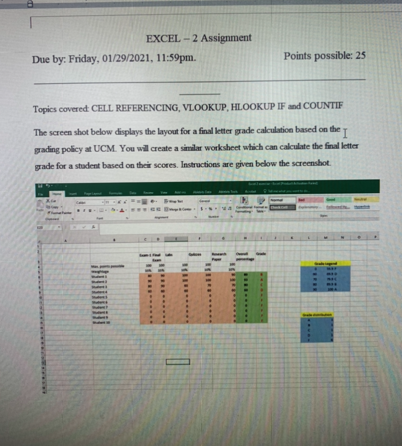
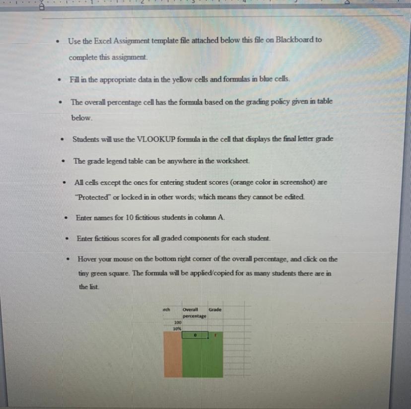
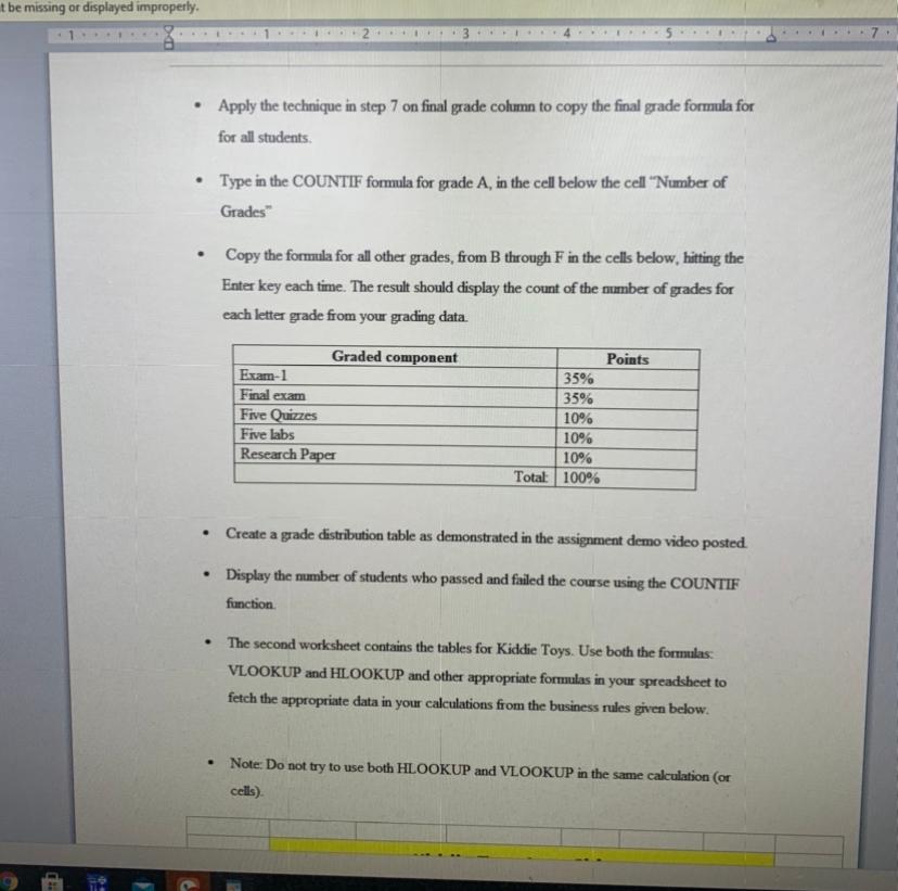
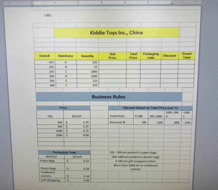
EXCEL - 2 Assignment Due by: Friday, 01/29/2021, 11:59pm. Points possible: 25 Topics covered: CELL REFERENCING, VLOOKUP, HLOOKUP IF and COUNTIF The screen shot below displays the layout for a final letter grade calculation based on the I grading policy at UCM. You will create a similar worksheet which can calculate the final letter grade for a student based on their scores. Instructions are given below the screenshot. Page Led X CU Good Neutral C Genew EE Merge Center S. Condial Fometas Check Foma Pune C 2 Research Piper Overall percentage 100 100 4 100 Gade end Mas ponts poste 100 3D SON 100 100 20 100 Student 7 14 . Use the Excel Assignment template file attached below this file on Blackboard to complete this assignment. Fill in the appropriate data in the yellow cells and formulas in blue cells. The overall percentage cell has the formula based on the grading policy given in table below Students will use the VLOOKUP formula in the cell that displays the final letter grade The grade legend table can be anywhere in the worksheet . All cells except the ones for entering student scores (orange color in screenshot) are "Protected" or locked in in other words; which means they cannot be edited. Enter names for 10 fictitious students in column A. Enter fictitious scores for all graded components for each student. Hover your mouse on the bottom right corner of the overall percentage, and click on the tiny green square. The formula will be applied copied for as many students there are in the list. wch Overall Grade percentage 100 1on 0 t be missing or displayed improperly. Apply the technique in step 7 on final grade column to copy the final grade formula for for all students Type in the COUNTIF formula for grade A, in the cell below the cell Number of Grades" Copy the formula for all other grades, from B through F in the cells below, hitting the Enter key each time. The result should display the count of the number of grades for each letter grade from your grading data. Graded component Exam-1 Final exam Five Quizzes Five Labs Research Paper Points 35% 35% 10% 10% 10% Total 100% Create a grade distribution table as demonstrated in the assignment demo video posted Display the mmber of students who passed and failed the course using the COUNTIF function The second worksheet contains the tables for Kiddie Toys. Use both the formulas VLOOKUP and HLOOKUP and other appropriate formulas in your spreadsheet to fetch the appropriate data in your calculations from the business rules given below. . Note: Do not try to use both HLOOKUP and VLOOKUP in the same calculation (or cells) 1 cells) Kiddie Toys Inc., China Orderd Distributor Quantity Unit Price Total Price Packaging costs Discount Grand Total 525 101 102 103 B D E 104 105 106 55 1800 2500 225 475 F Business Rules Price Discount based on Total Price (col. F) 1001-200 Total Price 0-500 501-1000 0 aty Sleach >200 1 Discount % 0% 15% 20% 25% 100 $ 500 $ 1000S 2000 $ 5.75 5.25 4.75 4.00 Packaging Costs Method Sleach Paper Bags $ 0.22 101 - 500 are packed in paper bags. 500-1000 are packed in plastic bags 0-100 are gift wrapped orders More than 1000 are in cardboard cartons us 0.28 Plastic Bags Cardboard Cartons Gift Wrapping S $ 0.18 0.30 EXCEL - 2 Assignment Due by: Friday, 01/29/2021, 11:59pm. Points possible: 25 Topics covered: CELL REFERENCING, VLOOKUP, HLOOKUP IF and COUNTIF The screen shot below displays the layout for a final letter grade calculation based on the I grading policy at UCM. You will create a similar worksheet which can calculate the final letter grade for a student based on their scores. Instructions are given below the screenshot. Page Led X CU Good Neutral C Genew EE Merge Center S. Condial Fometas Check Foma Pune C 2 Research Piper Overall percentage 100 100 4 100 Gade end Mas ponts poste 100 3D SON 100 100 20 100 Student 7 14 . Use the Excel Assignment template file attached below this file on Blackboard to complete this assignment. Fill in the appropriate data in the yellow cells and formulas in blue cells. The overall percentage cell has the formula based on the grading policy given in table below Students will use the VLOOKUP formula in the cell that displays the final letter grade The grade legend table can be anywhere in the worksheet . All cells except the ones for entering student scores (orange color in screenshot) are "Protected" or locked in in other words; which means they cannot be edited. Enter names for 10 fictitious students in column A. Enter fictitious scores for all graded components for each student. Hover your mouse on the bottom right corner of the overall percentage, and click on the tiny green square. The formula will be applied copied for as many students there are in the list. wch Overall Grade percentage 100 1on 0 t be missing or displayed improperly. Apply the technique in step 7 on final grade column to copy the final grade formula for for all students Type in the COUNTIF formula for grade A, in the cell below the cell Number of Grades" Copy the formula for all other grades, from B through F in the cells below, hitting the Enter key each time. The result should display the count of the number of grades for each letter grade from your grading data. Graded component Exam-1 Final exam Five Quizzes Five Labs Research Paper Points 35% 35% 10% 10% 10% Total 100% Create a grade distribution table as demonstrated in the assignment demo video posted Display the mmber of students who passed and failed the course using the COUNTIF function The second worksheet contains the tables for Kiddie Toys. Use both the formulas VLOOKUP and HLOOKUP and other appropriate formulas in your spreadsheet to fetch the appropriate data in your calculations from the business rules given below. . Note: Do not try to use both HLOOKUP and VLOOKUP in the same calculation (or cells) 1 cells) Kiddie Toys Inc., China Orderd Distributor Quantity Unit Price Total Price Packaging costs Discount Grand Total 525 101 102 103 B D E 104 105 106 55 1800 2500 225 475 F Business Rules Price Discount based on Total Price (col. F) 1001-200 Total Price 0-500 501-1000 0 aty Sleach >200 1 Discount % 0% 15% 20% 25% 100 $ 500 $ 1000S 2000 $ 5.75 5.25 4.75 4.00 Packaging Costs Method Sleach Paper Bags $ 0.22 101 - 500 are packed in paper bags. 500-1000 are packed in plastic bags 0-100 are gift wrapped orders More than 1000 are in cardboard cartons us 0.28 Plastic Bags Cardboard Cartons Gift Wrapping S $ 0.18 0.30