Excel Chapter $3$ Challenge Yourself $3\mathrm{.}4$

Purpose:

The objective of this assignment is to learn various Excel functions

that the student will apply to record data about completed and

planned college courses.

Skills needed to complete this project:

Finding Errors Using Trace Precedents and Trace Dependents $($Skill

$3\mathrm{.}21)$

Finding Data Using the VLOOKUP Function $($Skill $3\mathrm{.}18)$

Using the Function Arguments Dialog to Enter Functions $($Skill $3\mathrm{.}1)$

Checking Formulas for Errors $($Skill $3\mathrm{.}20)$

Creating Formulas Referencing Data from Other Worksheets $($Skill

$3\mathrm{.}11)$

Finding Data Using the XLOOKUP Function $($Skill $3\mathrm{.}19)$

Calculating Loan Payments Using the PMT Function $($Skill $3\mathrm{.}17)$

Using Date and Time Functions $($Skill $3\mathrm{.}5)$

Finding Minimum and Maximum Values $($Skill $3\mathrm{.}4)$

Using Formula AutoComplete to Enter Functions $($Skill $3\mathrm{.}2)$

Calculating Averages $($Skill $3\mathrm{.}3)$

Using the Logical Function IF $($Skill $3\mathrm{.}16)$

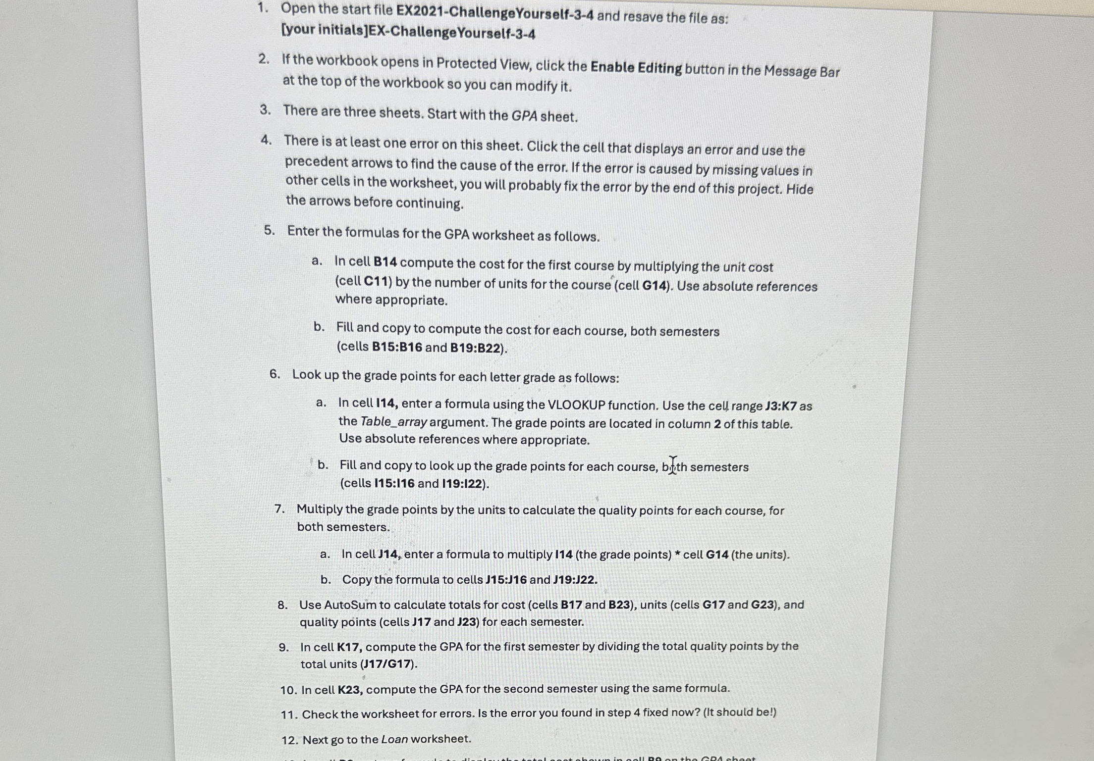
Open the start file EX$2021-$ChallengeYourself$-3-4$ and resave the file as:

$[$your initials$]$EX$-$ChallengeYourself$-3-4$

If the workbook opens in Protected View, click the Enable Editing button in the Message Bar

at the top of the workbook so you can modify it$.$

There are three sheets. Start with the GPA sheet.

There is at least one error on this sheet. Click the cell that displays an error and use the

precedent arrows to find the cause of the error. If the error is caused by missing values in

other cells in the worksheet, you will probably fix the error by the end of this project. Hide

the arrows before continuing.

Enter the formulas for the GPA worksheet as follows.

a$.$ In cell B$14$ compute the cost for the first course by multiplying the unit cost

$($cell C$11)$ by the number of units for the course $($cell G$14).$ Use absolute references

where appropriate.

b$.$ Fill and copy to compute the cost for each course, both semesters

$($cells B$15$:B$16$ and B$19$:B$22).$

Look up the grade points for each letter grade as follows:

a$.$ In cell I$14,$ enter a formula using the VLOOKUP function. Use the cell range J$3$:K$7$ as

the Table$\_$array argument. The grade points are located in column $2$ of this table.

Use absolute references where appropriate.

b$.$ Fill and copy to look up the grade points for each course, byith semesters

$($cells I$15$:I$16$ and I$19$:I$22).$

Multiply the grade points by the units to calculate the quality points for each course, for

both semesters.

a$.$ In cell J$14,$ enter a formula to multiply I$14($the grade points$)*$ cell G$14($the units$).$

b$.$ Copy the formula to cells J$15$:J$16$ and J$19$:J$22.$

Use AutoSum to calculate totals for cost $($cells B$17$ and B$23),$ units $($cells G$17$ and G$23),$ and

quality points $($cells $J17$ and $J23)$ for each semester.

In cell K$17,$ compute the GPA for the first semester by dividing the total quality points by the

total units $($J$17/$G$17).$

In cell K$23,$ compute the GPA for the second semester using the same formula.

Check the worksheet for errors. Is the error you found in step $4$ fixed now? $($It should be$!)$

Next go to the Loan worksheet.