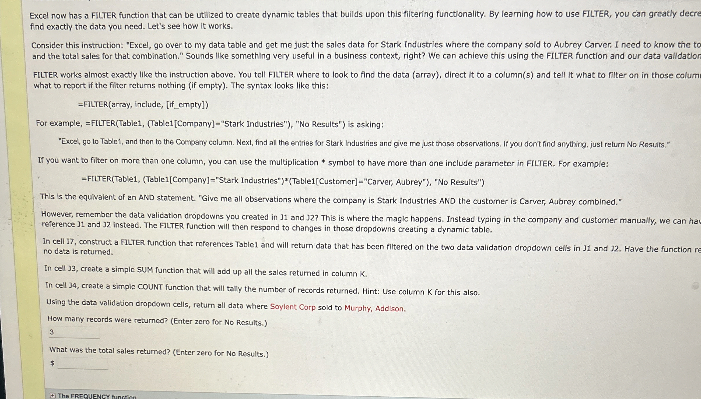
Question: Excel now has a FILTER function that can be utilized to create dynamic tables that builds upon this filtering functionality. By learning how to use
Excel now has a FILTER function that can be utilized to create dynamic tables that builds upon this filtering functionality. By learning how to use FILTER, you can greatly decre find exactly the data you need. Let's see how it works.
Consider this instruction: "Excel, go over to my data table and get me just the sales data for Stark Industries where the company sold to Aubrey Carver. I need to know the to and the total sales for that combination." Sounds like something very useful in a business context, right? We can achieve this using the FILTER function and our data validation
FILTER works almost exactly like the instruction above. You tell FILTER where to look to find the data array direct it to a columns and tell it what to filter on in those columi what to report if the filter returns nothing if empty The syntax looks like this:
FILTERarray include, ifempty
For example, FILTERTableTableCompany"Stark Industries"No Results" is asking:
"Excel, go to Table and then to the Company column. Next, find all the entries for Stark Industries and give me just those observations. If you don't find anything, just return No Results." If you want to filter on more than one column, you can use the multiplication symbol to have more than one include parameter in FILTER. For example:
FILTERTableTableCompany"Stark Industries"TableCustomer"Carver, Aubrey"No Results"
This is the equivalent of an AND statement. "Give me all observations where the company is Stark Industries AND the customer is Carver, Aubrey combined."
However, remember the data validation dropdowns you created in J and J This is where the magic happens. Instead typing in the company and customer manually, we can hav reference J and J instead. The FILTER function will then respond to changes in those dropdowns creating a dynamic table.
In cell I construct a FILTER function that references Table and will return data that has been filtered on the two data validation dropdown cells in J and J Have the function re no data is returned.
In cell J create a simple SUM function that will add up all the sales returned in column K
In cell J create a simple COUNT function that will tally the number of records returned. Hint: Use column for this also.
Using the data validation dropdown cells, return all data where Soylent Corp sold to Murphy, Addison.
How many records were returned? Enter zero for No Results.
What was the total sales returned? Enter zero for No Results.
$

Step by Step Solution
There are 3 Steps involved in it
1 Expert Approved Answer
Step: 1 Unlock


Question Has Been Solved by an Expert!
Get step-by-step solutions from verified subject matter experts
Step: 2 Unlock
Step: 3 Unlock


