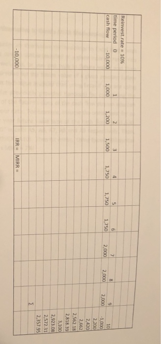
Excel's MIRR Alternative Calculation Instructions Use the following example, steps, and functions as an illustration of an alternative way Eyroll may be used to calculate the modified internal rate of return for a project. Step One: Place your data (see the attached example) in a time line format in Excel. Step Two: Using Excel's FV function solve for the future value of the cash flows as illustrated above, and place these future values in the cells below the last cash flow as illustrated above. Note: The first listed value (for us) is always the outlay cost and is never compounded. Step Three: Use Excel's SUM function to obtain the sum of the future values of the cash flows. Step Four: Use Excel's Zero coupon bond function to solve for the IRR=MIRR for the investment project. Zero Coupon Bond Function: The IRR provided by this function is the MIRR for these data. Assignment: Use the following data to solve for its MIRR: 70,000, 12,000, 15,000, 18,000, 21,000, 26,000. Use a compound rate of 5%. 10 Reinvest.rate = 10% time period 0 cash flow -10,000 1,200 1,500 1,000 1,750 1,750 1,750 2,000 2,000 2,000 2,200 2,420 2,662 2,562.18 2,818.39 3.100 2,923.08 2,572 31 2,357.95 IRR = MIRR = -10,000