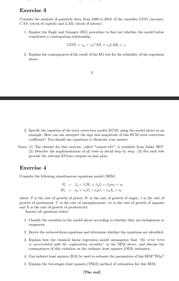
Question: Exercise 3 Consider the analysis of quarterly data, from 1980 to 2018, of the variables GDP (income), CAP (stock of capital) and LAB (stock of


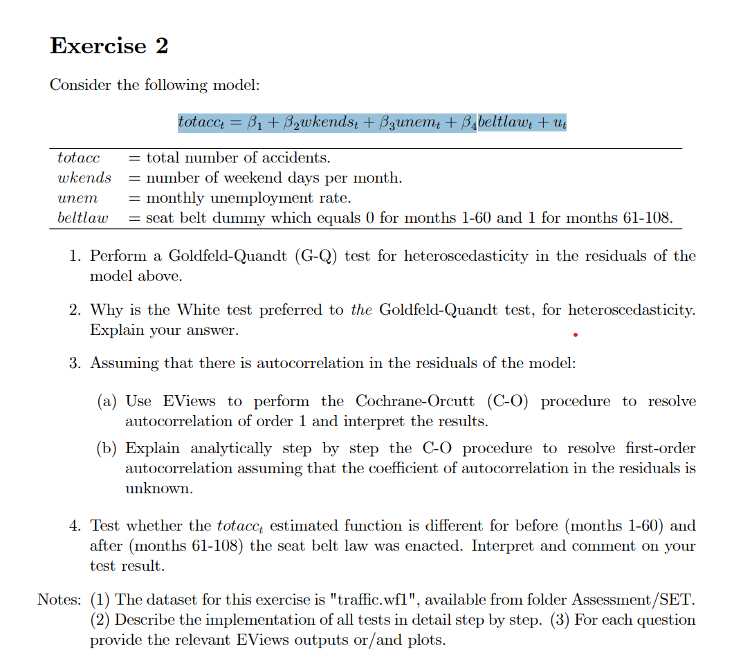
Exercise 3 Consider the analysis of quarterly data, from 1980 to 2018, of the variables GDP (income), CAP (stock of capital) and LAB (stock of labour). 1. Employ the Engle and Granger (EG) procedure to find out whether the model below constitutes a cointegrating relationship. GDP = %+ CAP + y2LAB: + 2. Explain the consequences of the result of the EG test for the reliability of the regression above. 3 3. Specify the equation of the error correction model (ECM) using the model above as an example. How can one interpret the sign and magnitude of this ECM error correction coefficient? You should use equations to illustrate your answer. Notes (1) The dataset for this exercise, called "output.wfl", is available from folder SET. (2) Describe the implementation of all tests in detail step by step. (3) For each test provide the relevant EViews outputs or/and plots. Exercise 4 Consider the following simultaneous equations model (SEM) P = B. +3,W4+3,12 + Bzime + ut W = 0 + 01P+Q2U. +3X+ 4 where P is the rate of growth of prices, W is the rate of growth of wages, I is the rate of growth of investment, U is the rate of unemployment, im is the rate of growth of imports and X is the rate of growth of productivity. Answer all questions below: 1. Classify the variables in the model above according to whether they are endogenous or exogenous. 2. Derive the reduced-form equations and determine whether the equations are identified. 3. Explain how the classical linear regression model assumption that "the error term is uncorrelated with the explanatory variables" in the SEM above, and discuss the consequences of this violation on the ordinary least squares (OLS) estimator. 4. Can indirect least squares (ILS) be used to estimate the parameters of this SEM? Why? 5. Explain the two-stages least squares (TSLS) method of estimation for this SEM. [The end Exercise 2 Consider the following model: totacct = B1 + B2wkendst + Bzunemt + Babeltlawt + ut totacc wkends beltlaw = total number of accidents. = number of weekend days per month. = monthly unemployment rate. = seat belt dummy which equals ( for months 1-60 and 1 for months 61-108. 1. Perform a Goldfeld-Quandt (G-Q) test for heteroscedasticity in the residuals of the model above. 2. Why is the White test preferred to the Goldfeld-Quandt test, for heteroscedasticity. Explain your answer. 3. Assuming that there is autocorrelation in the residuals of the model: (a) Use EViews to perform the Cochrane-Orcutt (C-0) procedure to resolve autocorrelation of order 1 and interpret the results. (b) Explain analytically step by step the C-O procedure to resolve first-order autocorrelation assuming that the coefficient of autocorrelation in the residuals is unknown. 4. Test whether the totacct estimated function is different for before (months 1-60) and after (months 61-108) the seat belt law was enacted. Interpret and comment on your test result. Notes: (1) The dataset for this exercise is "traffic.wfl", available from folder Assessment/SET. (2) Describe the implementation of all tests in detail step by step. (3) For each question provide the relevant EViews outputs or/and plots. Exercise 3 Consider the analysis of quarterly data, from 1980 to 2018, of the variables GDP (income), CAP (stock of capital) and LAB (stock of labour). 1. Employ the Engle and Granger (EG) procedure to find out whether the model below constitutes a cointegrating relationship. GDP = %+ CAP + y2LAB: + 2. Explain the consequences of the result of the EG test for the reliability of the regression above. 3 3. Specify the equation of the error correction model (ECM) using the model above as an example. How can one interpret the sign and magnitude of this ECM error correction coefficient? You should use equations to illustrate your answer. Notes (1) The dataset for this exercise, called "output.wfl", is available from folder SET. (2) Describe the implementation of all tests in detail step by step. (3) For each test provide the relevant EViews outputs or/and plots. Exercise 4 Consider the following simultaneous equations model (SEM) P = B. +3,W4+3,12 + Bzime + ut W = 0 + 01P+Q2U. +3X+ 4 where P is the rate of growth of prices, W is the rate of growth of wages, I is the rate of growth of investment, U is the rate of unemployment, im is the rate of growth of imports and X is the rate of growth of productivity. Answer all questions below: 1. Classify the variables in the model above according to whether they are endogenous or exogenous. 2. Derive the reduced-form equations and determine whether the equations are identified. 3. Explain how the classical linear regression model assumption that "the error term is uncorrelated with the explanatory variables" in the SEM above, and discuss the consequences of this violation on the ordinary least squares (OLS) estimator. 4. Can indirect least squares (ILS) be used to estimate the parameters of this SEM? Why? 5. Explain the two-stages least squares (TSLS) method of estimation for this SEM. [The end Exercise 2 Consider the following model: totacct = B1 + B2wkendst + Bzunemt + Babeltlawt + ut totacc wkends beltlaw = total number of accidents. = number of weekend days per month. = monthly unemployment rate. = seat belt dummy which equals ( for months 1-60 and 1 for months 61-108. 1. Perform a Goldfeld-Quandt (G-Q) test for heteroscedasticity in the residuals of the model above. 2. Why is the White test preferred to the Goldfeld-Quandt test, for heteroscedasticity. Explain your answer. 3. Assuming that there is autocorrelation in the residuals of the model: (a) Use EViews to perform the Cochrane-Orcutt (C-0) procedure to resolve autocorrelation of order 1 and interpret the results. (b) Explain analytically step by step the C-O procedure to resolve first-order autocorrelation assuming that the coefficient of autocorrelation in the residuals is unknown. 4. Test whether the totacct estimated function is different for before (months 1-60) and after (months 61-108) the seat belt law was enacted. Interpret and comment on your test result. Notes: (1) The dataset for this exercise is "traffic.wfl", available from folder Assessment/SET. (2) Describe the implementation of all tests in detail step by step. (3) For each question provide the relevant EViews outputs or/and plots
Step by Step Solution
There are 3 Steps involved in it

Get step-by-step solutions from verified subject matter experts


