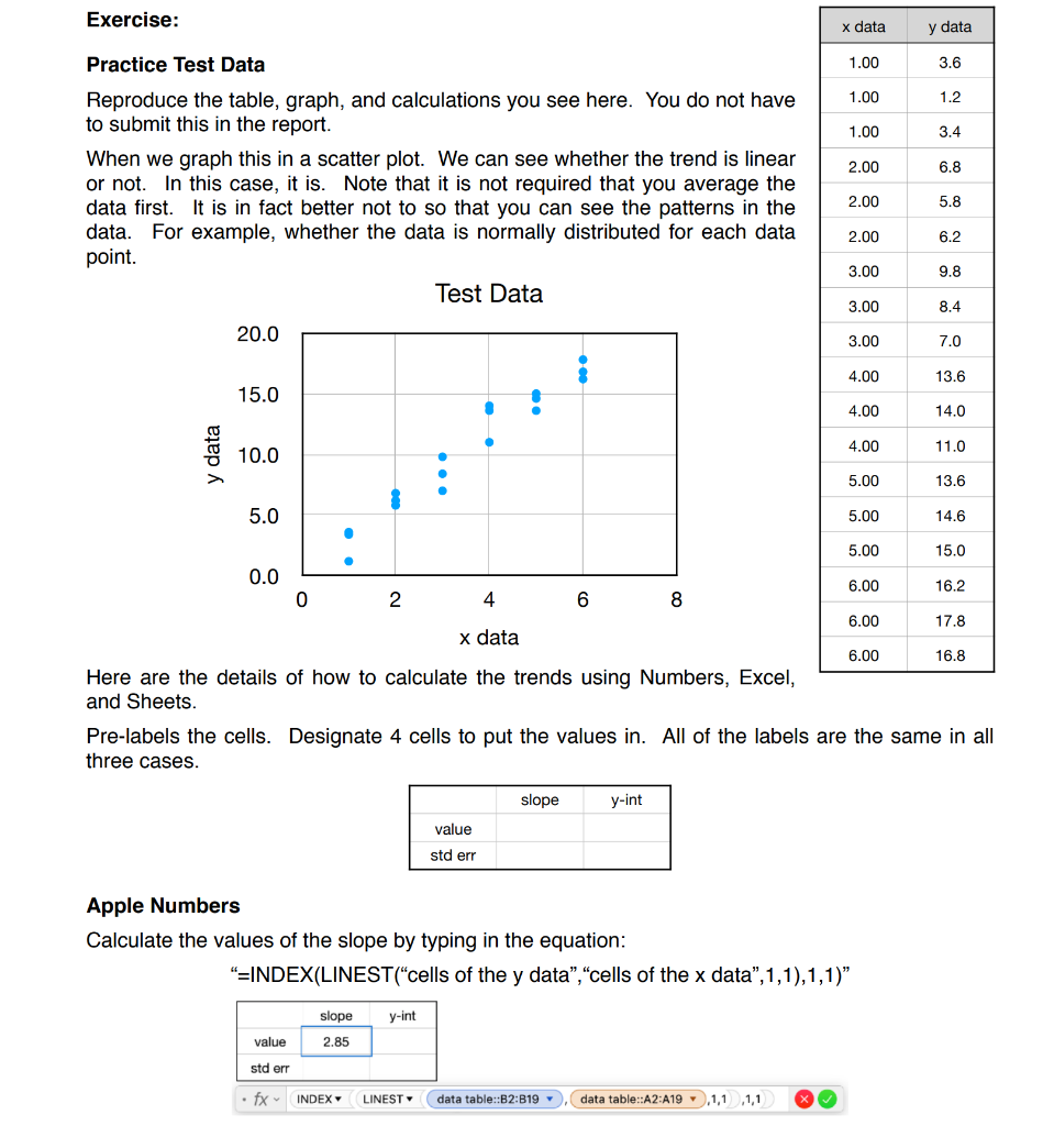
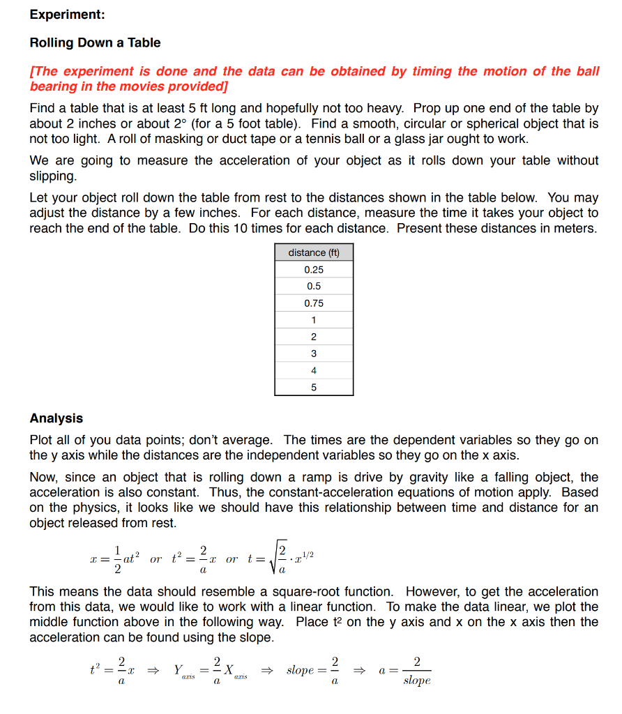
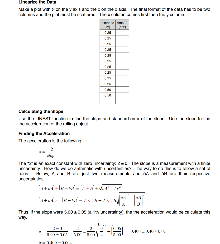
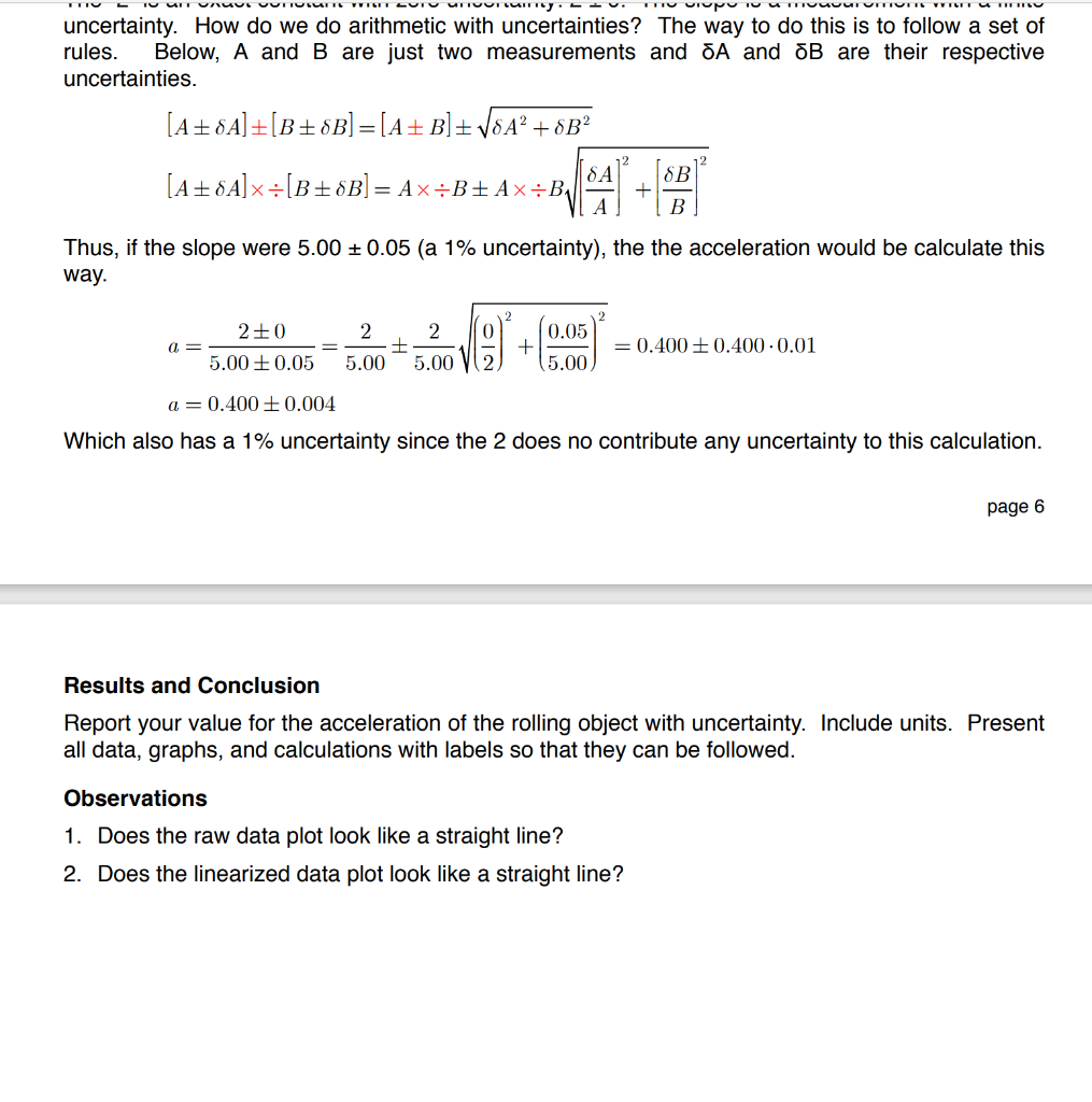
Exercise: x data y data Practice Test Data 1.00 3.6 1.00 1.2 1.00 3.4 2.00 6.8 Reproduce the table, graph, and calculations you see here. You do not have to submit this in the report. When we graph this in a scatter plot. We can see whether the trend is linear or not. In this case, it is. Note that it is not required that you average the data first. It is in fact better not to so that you can see the patterns in the data. For example, whether the data is normally distributed for each data point. Test Data 2.00 5.8 2.00 6.2 3.00 9.8 3.00 8.4 20.0 3.00 7.0 4.00 13.6 15.0 4.00 14.0 data 10.0 4.00 11.0 5.00 13.6 6.00 5.0 5.00 14.6 . 5.00 15.0 0.0 6.00 16.2 0 2 4 6 8 17.8 x data 6.00 16.8 Here are the details of how to calculate the trends using Numbers, Excel, and Sheets. Pre-labels the cells. Designate 4 cells to put the values in. All of the labels are the same in all three cases. slope y-int value std err Apple Numbers Calculate the values of the slope by typing in the equation: =INDEX(LINEST("cells of the y data", "cells of the x data",1,1),1,1)" slope y-int value 2.85 std err fx INDEX LINEST data table::B2:B19 data table::A2:A19.1,1 1,1 Experiment: Rolling Down a Table [The experiment is done and the data can be obtained by timing the motion of the ball bearing in the movies provided] Find a table that is at least 5 ft long and hopefully not too heavy. Prop up one end of the table by about 2 inches or about 2 (for a 5 foot table). Find a smooth, circular or spherical object that is not too light. A roll masking or duct tape or a tennis ball or a glass jar ought to work. We are going to measure the acceleration of your object as it rolls down your table without slipping. Let your object roll down the table from rest to the distances shown in the table below. You may adjust the distance by a few inches. For each distance, measure the time it takes your object to reach the end of the table. Do this 10 times for each distance. Present these distances in meters. distance (ft) 0.25 0.5 0.75 1 2 3 4 5 Analysis Plot all of you data points, don't average. The times are the dependent variables so they go on the y axis while the distances are the independent variables so they go on the x axis. Now, since an object that is rolling down a ramp is drive by gravity like a falling object, the acceleration is also constant. Thus, the constant acceleration equations of motion apply. Based on the physics, it looks like we should have this relationship between time and distance for an object released from rest. or t2 = . | = = or -- 1/2 This means the data should resemble a square-root function. However, to get the acceleration from this data, we would like to work with a linear function. To make the data linear, we plot the middle function above in the following way. Place t2 on the y axis and x on the x axis then the acceleration can be found using the slope. 2 = 22 Y 2 X a 2 slope = a a a slope Linearize the Data Make a plot with t2 on the y axis and the x on the x axis. The final format of the data has to be two columns and the plot must be scattered. The x column comes first then the y column. distance time12 (m) (s^2) 0.25 0.25 0.25 0.25 0.25 0.25 0.25 0.25 0.25 0.25 0.50 0.50 Calculating the Slope Use the LINEST function to find the slope and standard error of the slope. Use the slope to find the acceleration of the rolling object. Finding the Acceleration The acceleration is the following. 2 a = slope The 2 is an exact constant with zero uncertainty: 2 +0. The slope is a measurement with a finite uncertainty. How do we do arithmetic with uncertainties? The way to do this is to follow a set of rules. Below, A and B are just two measurements and OA and 5B are their respective uncertainties. (A 8A]+[B+ SB] =[A + B]VOA+8B? SA (SB [A + 8A]=(B8B]=AxB+ Ax=B, B Thus, if the slope were 5.00 + 0.05 (a 1% uncertainty), the the acceleration would be calculate this way. 0 a = 2 +0 5.00 +0.05 2 2 + 5.00 5.00 + 0.05 5.00 = 0.400 + 0.400.0.01 a 0.400 +0.004 uncertainty. How do we do arithmetic with uncertainties? The way to do this is to follow a set of rules. Below, A and B are just two measurements and 5A and JB are their respective uncertainties. [A+8A]+[B+8B]=[A+B] + 16A +8B (A+8A]x-[B+8B] = AX=BAXBA SA SB + B Thus, if the slope were 5.00+ 0.05 (a 1% uncertainty), the the acceleration would be calculate this way. 2 +0 a= 5.00+ 0.05 2 2 + 5.00 5.00 0.05 5.00 = 0.400 0.400.0.01 a=0.400 + 0.004 Which also has a 1% uncertainty since the 2 does no contribute any uncertainty to this calculation. page 6 Results and Conclusion Report your value for the acceleration of the rolling object with uncertainty. Include units. Present all data, graphs, and calculations with labels so that they can be followed. Observations 1. Does the raw data plot look like a straight line? 2. Does the linearized data plot look like a straight line? Exercise: x data y data Practice Test Data 1.00 3.6 1.00 1.2 1.00 3.4 2.00 6.8 Reproduce the table, graph, and calculations you see here. You do not have to submit this in the report. When we graph this in a scatter plot. We can see whether the trend is linear or not. In this case, it is. Note that it is not required that you average the data first. It is in fact better not to so that you can see the patterns in the data. For example, whether the data is normally distributed for each data point. Test Data 2.00 5.8 2.00 6.2 3.00 9.8 3.00 8.4 20.0 3.00 7.0 4.00 13.6 15.0 4.00 14.0 data 10.0 4.00 11.0 5.00 13.6 6.00 5.0 5.00 14.6 . 5.00 15.0 0.0 6.00 16.2 0 2 4 6 8 17.8 x data 6.00 16.8 Here are the details of how to calculate the trends using Numbers, Excel, and Sheets. Pre-labels the cells. Designate 4 cells to put the values in. All of the labels are the same in all three cases. slope y-int value std err Apple Numbers Calculate the values of the slope by typing in the equation: =INDEX(LINEST("cells of the y data", "cells of the x data",1,1),1,1)" slope y-int value 2.85 std err fx INDEX LINEST data table::B2:B19 data table::A2:A19.1,1 1,1 Experiment: Rolling Down a Table [The experiment is done and the data can be obtained by timing the motion of the ball bearing in the movies provided] Find a table that is at least 5 ft long and hopefully not too heavy. Prop up one end of the table by about 2 inches or about 2 (for a 5 foot table). Find a smooth, circular or spherical object that is not too light. A roll masking or duct tape or a tennis ball or a glass jar ought to work. We are going to measure the acceleration of your object as it rolls down your table without slipping. Let your object roll down the table from rest to the distances shown in the table below. You may adjust the distance by a few inches. For each distance, measure the time it takes your object to reach the end of the table. Do this 10 times for each distance. Present these distances in meters. distance (ft) 0.25 0.5 0.75 1 2 3 4 5 Analysis Plot all of you data points, don't average. The times are the dependent variables so they go on the y axis while the distances are the independent variables so they go on the x axis. Now, since an object that is rolling down a ramp is drive by gravity like a falling object, the acceleration is also constant. Thus, the constant acceleration equations of motion apply. Based on the physics, it looks like we should have this relationship between time and distance for an object released from rest. or t2 = . | = = or -- 1/2 This means the data should resemble a square-root function. However, to get the acceleration from this data, we would like to work with a linear function. To make the data linear, we plot the middle function above in the following way. Place t2 on the y axis and x on the x axis then the acceleration can be found using the slope. 2 = 22 Y 2 X a 2 slope = a a a slope Linearize the Data Make a plot with t2 on the y axis and the x on the x axis. The final format of the data has to be two columns and the plot must be scattered. The x column comes first then the y column. distance time12 (m) (s^2) 0.25 0.25 0.25 0.25 0.25 0.25 0.25 0.25 0.25 0.25 0.50 0.50 Calculating the Slope Use the LINEST function to find the slope and standard error of the slope. Use the slope to find the acceleration of the rolling object. Finding the Acceleration The acceleration is the following. 2 a = slope The 2 is an exact constant with zero uncertainty: 2 +0. The slope is a measurement with a finite uncertainty. How do we do arithmetic with uncertainties? The way to do this is to follow a set of rules. Below, A and B are just two measurements and OA and 5B are their respective uncertainties. (A 8A]+[B+ SB] =[A + B]VOA+8B? SA (SB [A + 8A]=(B8B]=AxB+ Ax=B, B Thus, if the slope were 5.00 + 0.05 (a 1% uncertainty), the the acceleration would be calculate this way. 0 a = 2 +0 5.00 +0.05 2 2 + 5.00 5.00 + 0.05 5.00 = 0.400 + 0.400.0.01 a 0.400 +0.004 uncertainty. How do we do arithmetic with uncertainties? The way to do this is to follow a set of rules. Below, A and B are just two measurements and 5A and JB are their respective uncertainties. [A+8A]+[B+8B]=[A+B] + 16A +8B (A+8A]x-[B+8B] = AX=BAXBA SA SB + B Thus, if the slope were 5.00+ 0.05 (a 1% uncertainty), the the acceleration would be calculate this way. 2 +0 a= 5.00+ 0.05 2 2 + 5.00 5.00 0.05 5.00 = 0.400 0.400.0.01 a=0.400 + 0.004 Which also has a 1% uncertainty since the 2 does no contribute any uncertainty to this calculation. page 6 Results and Conclusion Report your value for the acceleration of the rolling object with uncertainty. Include units. Present all data, graphs, and calculations with labels so that they can be followed. Observations 1. Does the raw data plot look like a straight line? 2. Does the linearized data plot look like a straight line