

Question: Exercises 1 . Copy your code into another cell, and modify to plot the 1 0 th order Taylor series approximation and theoretical error of
Exercises
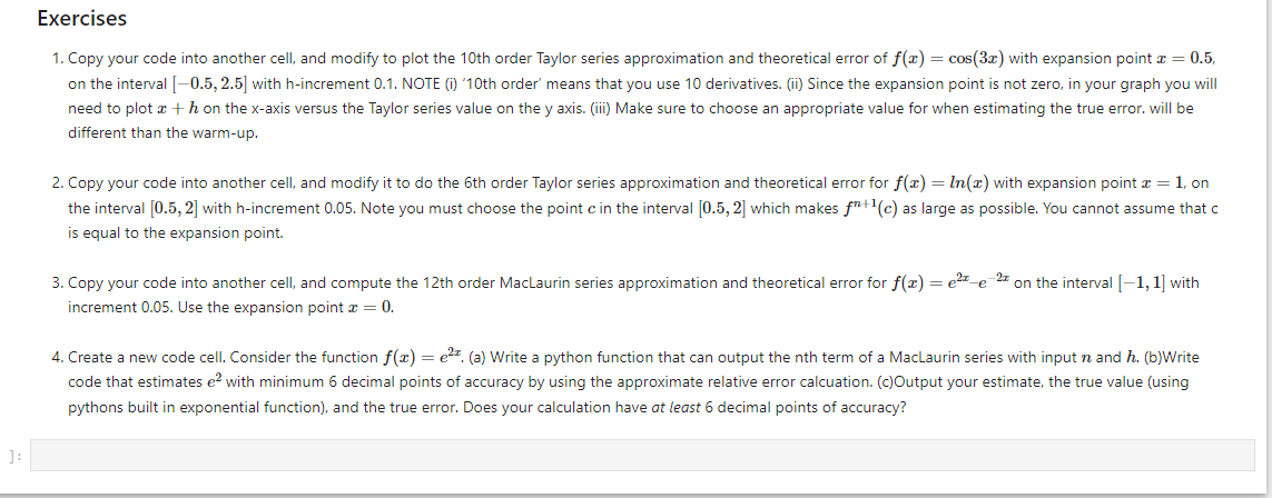
Copy your code into another cell, and modify to plot the th order Taylor series approximation and theoretical error of with expansion point
on the interval with hincrement NOTE ith order' means that you use derivatives. ii Since the expansion point is not zero, in your graph you will
need to plot on the axis versus the Taylor series value on the axis. iii Make sure to choose an appropriate value for when estimating the true error. will be
different than the warmup
Copy your code into another cell, and modify it to do the th order Taylor series approximation and theoretical error for with expansion point on
the interval with hincrement Note you must choose the point in the interval which makes as large as possible. You cannot assume that c
is equal to the expansion point.
Copy your code into another cell, and compute the th order MacLaurin series approximation and theoretical error for on the interval with
increment Use the expansion point
Create a new code cell. Consider the function a Write a python function that can output the nth term of a MacLaurin series with input and bWrite
code that estimates with minimum decimal points of accuracy by using the approximate relative error calcuation. cOutput your estimate, the true value using
pythons built in exponential function and the true error. Does your calculation have at least decimal points of accuracy? This is the original code and it must be change to be able to be able to work with the exercises in different codes import numpy as np
import matplotlib.pyplot as plt
matplotlib inline
# Factorial comes from 'math' package
from math import factorial
#
### Initialize section
#array of derivatives at compute by hand
deriv nparray
# degree of Taylor polynomial
Nlenderiv
# Max abs value of N deriv on interval Compute using calculus
# used in error formula: error abshNN maxabsNth deriv.
maxAbsNplusderiv
#array with h values
h nparange
# Give the expansion point for the Taylor series
expansion
# Create an array to contain Taylor series
taylornpzeroslenh
#
### Calculation section
#calculate Taylor series for all h at once using a loop
for n in rangeN:
taylor taylor hnfactorialnderivn
#actual function values
actualFn npcosexpansionh
#error actual and taylor series
actualAbsError abstayloractualFn
#theoretical errorhdegdegmaxn deriv
theoAbsError abshNfactorialNmaxAbsNplusderiv
#Compute actual x values displaced by expansion point
xActual expansionh
#
### Output section
#plot figures for cos and errors using
# Objectoriented style plotting
# Two subplots in a row
fig, axes pltsubplotsnrows ncols figsize
# objects for the left subplot attached to axes #
axesplotxActual taylor, rlabel"Taylor series"
axesplotxActual actualFn, b label"Cosx
axeslegendloc #legend in upper left
axessettitleTaylor Series for cosx
# objects for the right subplot attached to axes #
axesplotxActual actualAbsError, label"Actual Absolute Error"
axesplotxActual theoAbsError, label"Theoretical Absolute Error"
axeslegendloc #legend in upper left
axessettitleActual and Theoretical Error"
Step by Step Solution
There are 3 Steps involved in it
1 Expert Approved Answer
Step: 1 Unlock

Question Has Been Solved by an Expert!
Get step-by-step solutions from verified subject matter experts
Step: 2 Unlock
Step: 3 Unlock