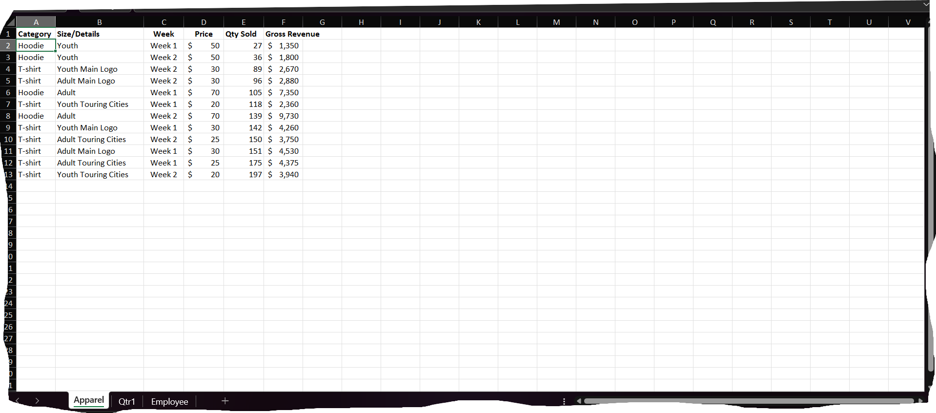
Exp$22\_$Excel$\_$Ch$05\_$Cumulative$\_$Merchandise $1\mathrm{.}1$ Project Description: You manage the souvenir shop for a touring Broadway production. The shop sells apparel, souvenirs, and media items. You created datasets to analyze sales in the different categories. One sheet contains apparel sales for the first two weeks of the month. You will insert subtotal rows in this worksheet. The second sheet contains product information for the first quarter of the year. You will create a PivotTable, insert a timeline, and create a PivotChart using this data. You will create a second PivotTable so that you can filter data and calculate product prices if you run a sale. Finally, the last sheet contains two tables containing employee data. You will create a relationship and then create a PivotTable using that data. Steps to Perform: Step Instructions Points Possible $1$ Start Excel. Download and open the file named Exp$22\_$Excel$\_$Ch$05\_$Cumulative$\_$Merchandise.xlsx$.$ Grader has automatically added your last name to the beginning of the filename. $02$ Your first task is to sort the dataset on the Apparel worksheet. Ensure the Apparel worksheet is active. Sort the data by Week in alphabetical order and further sort it by Category in alphabetical order. $33$ You want to focus on apparel sales within one month. You will insert subtotal rows to display total sales by week $(1$ and $2)$ and by category $($Hoodie and T$-$shirt$).$ Use the Subtotal feature to insert subtotal rows by Week to calculate the totals for Qty Sold and Gross Revenue. Add a second subtotal $($without removing the first subtotal by Category to calculate the totals for Qty Sold and Gross Revenue. $54$ To focus on the Gross Revenue, you will apply an outline and collapse columns. Create an automatic outline and collapse the outline above Gross Revenue. $35$ Next, you want to create a blank PivotTable and then name it$.$ Display the Qtr$1$ worksheet and create a blank PivotTable on a new worksheet. Do not add data to the data model. Name the PivotTable Qtr$1$ Sales. Change the name of the worksheet to Sales PivotTable. $56$ The PivotTable should determine total number of items sold and the total gross revenue by category for the first quarter. Place the Category field in rows. Place the Gross Revenue and Qty Sold fields as values. $57$ You will format the values in the PivotTable to look more professional and change the custom names that display as column headings. Modify the Sum of Gross Revenue field with the custom name Total Gross Revenue and apply Accounting Number Format with $0$ decimal places. $38$ Modify the Sum of Qty Sold field with the custom name Total Qty Sold, apply Number format with $0$ decimal places, and select the Use $1000$ Separator $(,)$ option $49$ Now you want to insert a timeline so that you can filter the PivotTable by month. Insert a timeline for the Month field. Click or select March to filter the PivotTable to display only March data. Cut the timeline and paste it in cell A$9.$ Set the timeline width to $3\mathrm{.}3$ inches. $410$ You want to create a PivotChart to display percentages in a pie chart. Insert a PivotChart pie chart that depicts the categories and gross revenue. Cut the chart and paste it in cell D$1.511$ Next, you want to remove the legend and display data labels. Remove the legend. Display data labels in the best fit position with only the Category Name and Percentage labels. $412$ You are ready to finish the PivotChart by adding a title and changing the width. Change the title to Gross Revenue. Change the chart width to $3\mathrm{.}9$ inches. $313$ Extracting a value from the PivotTable and displaying it on the main worksheet is helpful as you look through the dataset. Click or select cell H$1$ in the Qtr$1$ worksheet. Insert the GETPIVOTDATA function to retrieve the grand total in the Total Gross Revenue column in the filtered PivotTable. $514$ Next, you want to create a recommended PivotTable to analyze product sales in the Apparel category. Use the data on the Qtr$1$ worksheet to create a recommended PivotTable using the Sum of Retail Price by Category. Name the PivotTable Sale Prices. Change the name of the worksheet to Sale Prices. $415$ Move the Category field from the Rows area to Filters area. Add the Product field to the Rows area. Modify the Sum of Retail Price field with the custom name Item Retail Price and apply Accounting format with zero decimal places. $616$ Now you want to focus on only the Souvenirs data. Set a filter to display on the Souvenirs category. $517$ You will create a calculated field to determine product retail prices if you offer a $15\%$ sale, which is $85\%$ of the current retail price. Create a calculated field using the default name Field$1$ to multiply the Retail Price by $\mathrm{.}85.$ Modify the calculated field with the custom name Sale Price and apply Accounting Number Format with zero decimal places. $318$ Next, you will apply a different PivotTable style to have a similar color scheme as the dataset. $\backslash$begin$\{$tabular$\}\{|$c$|$c$|$c$|$c$|$c$|$c$|$c$|$c$|$c$|$c$|$c$|$c$|$c$|$c$|$c$|$c$|$c$|$c$|$c$|$c$|$c$|$c$|$c$|\}$