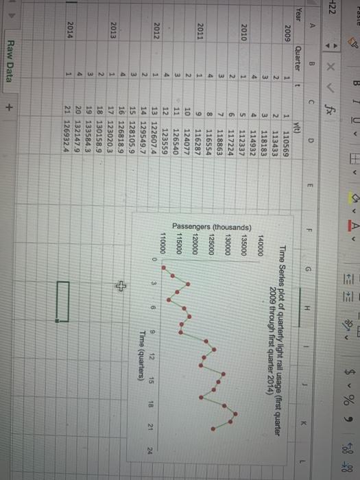
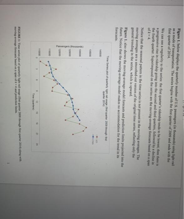
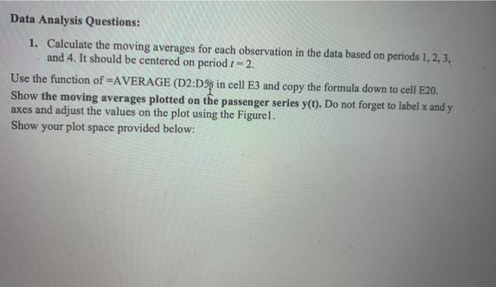
Faste 1 NE & A $ % 9 68 H22 X B D E F G H 1 K Year t Quarter 2009 1 2 Time Series plot of quarterly light rail usage (first quarter 2009 through first quarter 2014) 140000 3 4 2010 135000 2 130000 3 4 Passengers (thousands) 125000 2011 1 120000 yt) 1 110569 2 113433 3 118183 4 114932 5 112337 6 117224 7 118863 8 116554 9 116287 10 124077 126540 123559 13 122607.4 14 129549.7 15 128105.9 16 126818.9 17 123020.3 18 130158.9 19 133584.3 20 132147.9 21 126932.4 115000 11 12 2 3 4 1 2 3 2012 110000 0 3 6 18 21 24 9 12 15 Time (quarters) 2013 1 2 3 4 2014 1 Raw Data + Figure 1 below displays the quarterly number of U.S. passengers (in thousands) using light rail as a mode of transportation. The series begins with the first quarter of 2009 and ends with the first quarter of 2014 We can see a regularity to the series: the first quarter's ridership tends to be lowest; then there is a progressive rise in ridership going into the second and third quarters, followed by a decline in the fourth quarter. Superimposed on the series are the moving-average forecasts based on a span ofk-4. Notice that the seasonal pattern in the time series is not present in the moving averages. The moving averages are a smoothed-out version of the original time series, reflecting only the general trending in the series, which is upward. Figure 1. also shows the moving-average model forecasts and prediction limits projected into the future. Notice that the moving average model makes no accommodation for the trend in its forecasts. Time Series plot of quarterly light rail usage (first quarter 2009 through first quarter 2014) 160000 . - 135000 150000 Passengers (thousands) 125000 120000 115000 110000 24 15 Time (quarters) FIGURE 1: Time series plot of quarterly light rail usage (first quarter 2009 through fint quarter 2014) along with moving average forecasts based on a span of k-4 and prediction limits. Data Analysis Questions: 1. Calculate the moving averages for each observation in the data based on periods 1, 2, 3, and 4. It should be centered on period t= 2. Use the function of =AVERAGE (D2:DSi in cell E3 and copy the formula down to cell E20. Show the moving averages plotted on the passenger series y(t). Do not forget to label x and y axes and adjust the values on the plot using the Figurel. Show your plot space provided below: Faste 1 NE & A $ % 9 68 H22 X B D E F G H 1 K Year t Quarter 2009 1 2 Time Series plot of quarterly light rail usage (first quarter 2009 through first quarter 2014) 140000 3 4 2010 135000 2 130000 3 4 Passengers (thousands) 125000 2011 1 120000 yt) 1 110569 2 113433 3 118183 4 114932 5 112337 6 117224 7 118863 8 116554 9 116287 10 124077 126540 123559 13 122607.4 14 129549.7 15 128105.9 16 126818.9 17 123020.3 18 130158.9 19 133584.3 20 132147.9 21 126932.4 115000 11 12 2 3 4 1 2 3 2012 110000 0 3 6 18 21 24 9 12 15 Time (quarters) 2013 1 2 3 4 2014 1 Raw Data + Figure 1 below displays the quarterly number of U.S. passengers (in thousands) using light rail as a mode of transportation. The series begins with the first quarter of 2009 and ends with the first quarter of 2014 We can see a regularity to the series: the first quarter's ridership tends to be lowest; then there is a progressive rise in ridership going into the second and third quarters, followed by a decline in the fourth quarter. Superimposed on the series are the moving-average forecasts based on a span ofk-4. Notice that the seasonal pattern in the time series is not present in the moving averages. The moving averages are a smoothed-out version of the original time series, reflecting only the general trending in the series, which is upward. Figure 1. also shows the moving-average model forecasts and prediction limits projected into the future. Notice that the moving average model makes no accommodation for the trend in its forecasts. Time Series plot of quarterly light rail usage (first quarter 2009 through first quarter 2014) 160000 . - 135000 150000 Passengers (thousands) 125000 120000 115000 110000 24 15 Time (quarters) FIGURE 1: Time series plot of quarterly light rail usage (first quarter 2009 through fint quarter 2014) along with moving average forecasts based on a span of k-4 and prediction limits. Data Analysis Questions: 1. Calculate the moving averages for each observation in the data based on periods 1, 2, 3, and 4. It should be centered on period t= 2. Use the function of =AVERAGE (D2:DSi in cell E3 and copy the formula down to cell E20. Show the moving averages plotted on the passenger series y(t). Do not forget to label x and y axes and adjust the values on the plot using the Figurel. Show your plot space provided below