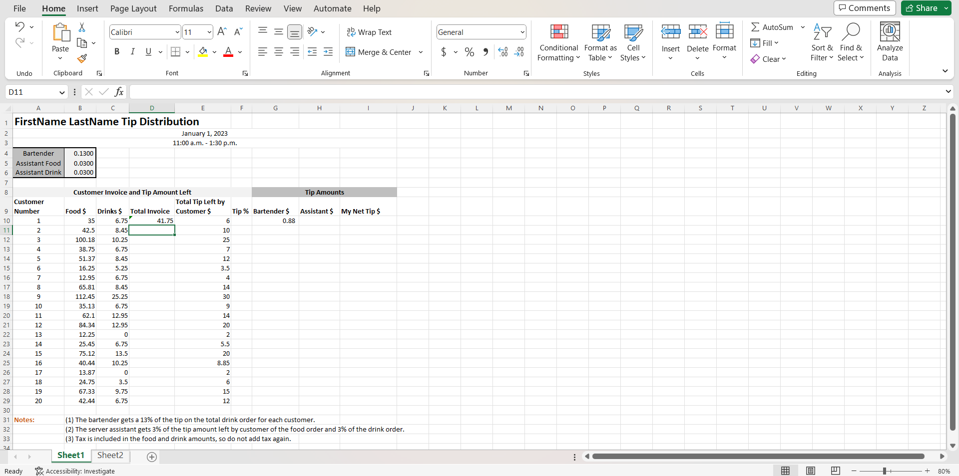
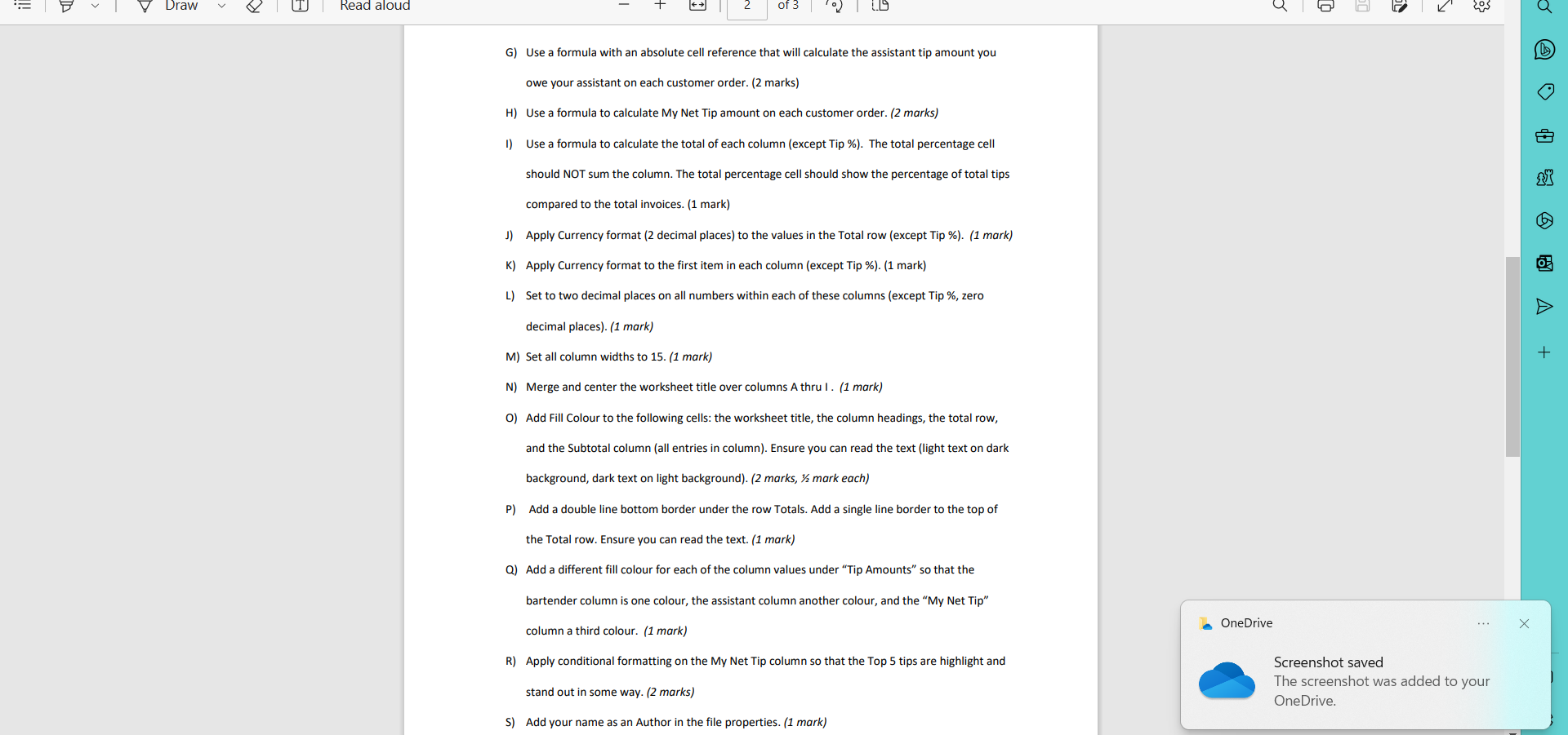
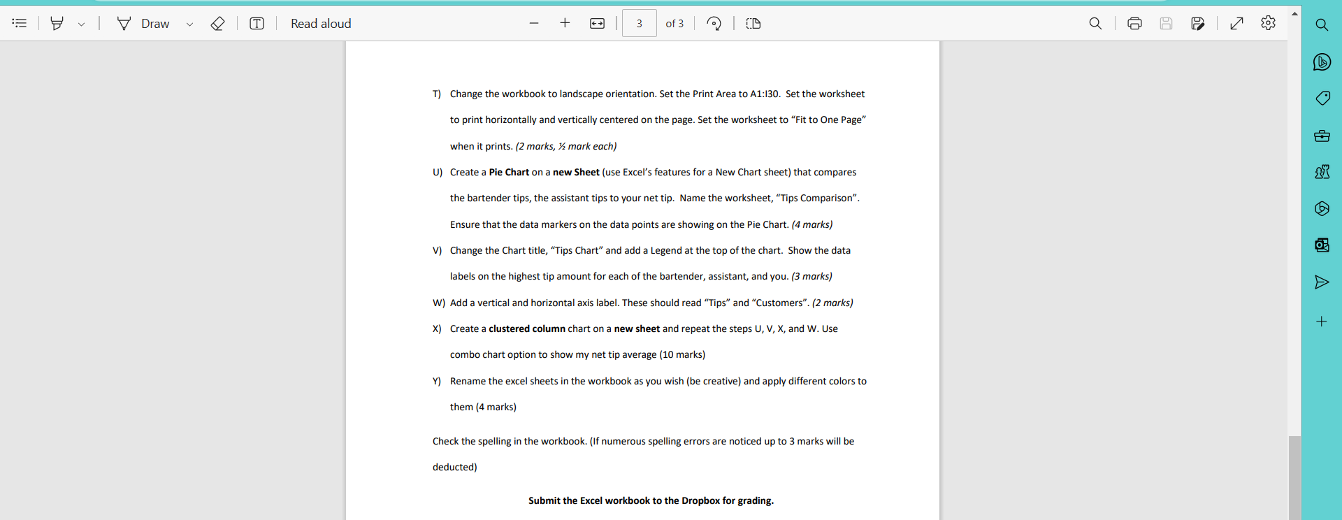
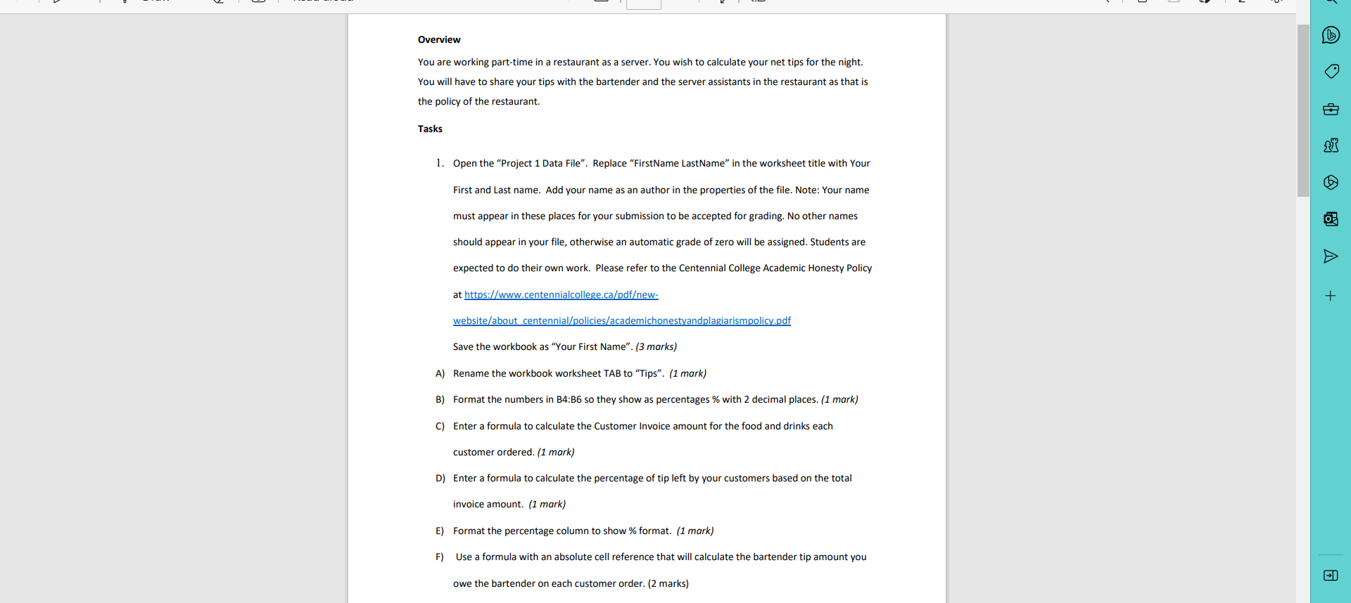
File Home Insert Page Layout Formulas Data Review View Automate Help Comments Share Calibri 11 A" A ab Wrap Text General AutoSum AY O Fill Paste E Merge & Center $ ~ % " Conditional Format as Cell Insert Delete Format Sort & Find & Analyze Formatting * Table Styles v Clear Filter ~ Select Data Undo Clipboard Font Alignment Number Styles Cells Editing Analysis D11 vi XVfx C E F G H K M N O P Q R S T U V W X Y Z FirstName LastName Tip Distribution January 1, 2023 AWN 11:00 a.m. - 1:30 p.m. Bartender 0.1300 Assistant Food 0.0300 Assistant Drink 0.0300 Customer Invoice and Tip Amount Left Tip Amounts Customer Total Tip Left by Number Food $ Drinks $ Total Invoice Customer $ Tip % Bartender $ Assistant $ My Net Tip $ 10 35 6.75 41.75 6 0.88 42.5 8.45 10 12 100.18 10.25 25 13 38.75 6.75 7 14 51.37 8.45 12 15 16.25 5.25 3.5 16 12.95 6.75 4 17 8 65.81 8.45 14 18 112.45 25.25 30 19 10 35.13 6.75 9 20 11 62.1 12.95 14 12 84.34 12.95 20 13 12.25 2 14 25.45 6.75 5.5 15 75.12 13.5 20 25 16 40.44 10.25 8.85 26 17 13.87 27 18 24.75 3.5 28 19 67.33 9.75 15 29 20 42.44 6.75 12 30 31 Notes: (1) The bartender gets a 13% of the tip on the total drink order for each customer. 32 (2) The server assistant gets 3% of the tip amount left by customer of the food order and 3% of the drink order. 33 3) Tax is included in the food and drink amounts, so do not add tax again. 24 Sheet1 Sheet2 + Ready Accessibility: Investigate - 80%Draw | Read aloud of 3 G) Use a formula with an absolute cell reference that will calculate the assistant tip amount you owe your assistant on each customer order. (2 marks) H) Use a formula to calculate My Net Tip amount on each customer order. (2 marks) 1) Use a formula to calculate the total of each column (except Tip %). The total percentage cell should NOT sum the column. The total percentage cell should show the percentage of total tips compared to the total invoices. (1 mark) J) Apply Currency format (2 decimal places) to the values in the Total row (except Tip %). (1 mark) K) Apply Currency format to the first item in each column (except Tip %). (1 mark) L) Set to two decimal places on all numbers within each of these columns (except Tip %, zero decimal places). (1 mark) M) Set all column widths to 15. (1 mark) + N) Merge and center the worksheet title over columns A thru I . (1 mark) O) Add Fill Colour to the following cells: the worksheet title, the column headings, the total row, and the Subtotal column (all entries in column). Ensure you can read the text (light text on dark background, dark text on light background). (2 marks, y mark each) P) Add a double line bottom border under the row Totals. Add a single line border to the top of the Total row. Ensure you can read the text. (1 mark) Q) Add a different fill colour for each of the column values under "Tip Amounts" so that the bartender column is one colour, the assistant column another colour, and the "My Net Tip" OneDrive . . . column a third colour. (1 mark) X R) Apply conditional formatting on the My Net Tip column so that the Top 5 tips are highlight and Screenshot saved The screenshot was added to your stand out in some way. (2 marks) OneDrive. S) Add your name as an Author in the file properties. (1 mark)Draw Read aloud + 3 of 3 So3 Q T) Change the workbook to landscape orientation. Set the Print Area to A1:130. Set the worksheet to print horizontally and vertically centered on the page. Set the worksheet to "Fit to One Page" when it prints. (2 marks, % mark each) U) Create a Pie Chart on a new Sheet (use Excel's features for a New Chart sheet) that compares the bartender tips, the assistant tips to your net tip. Name the worksheet, "Tips Comparison". Ensure that the data markers on the data points are showing on the Pie Chart. (4 marks) V) Change the Chart title, "Tips Chart" and add a Legend at the top of the chart. Show the data labels on the highest tip amount for each of the bartender, assistant, and you. (3 marks) W) Add a vertical and horizontal axis label. These should read "Tips" and "Customers". (2 marks) + X) Create a clustered column chart on a new sheet and repeat the steps U, V, X, and W. Use combo chart option to show my net tip average (10 marks) Y) Rename the excel sheets in the workbook as you wish (be creative) and apply different colors to them (4 marks) Check the spelling in the workbook. (If numerous spelling errors are noticed up to 3 marks will be deducted) Submit the Excel workbook to the Dropbox for grading.Overview You are working part-time in a restaurant as a server. You wish to calculate your net tips for the night. You will have to share your tips with the bartender and the server assistants in the restaurant as that is the policy of the restaurant. Tasks 1. Open the "Project 1 Data File". Replace "FirstName LastName" in the worksheet title with Your First and Last name. Add your name as an author in the properties of the file. Note: Your name must appear in these places for your submission to be accepted for grading. No other names should appear in your file, otherwise an automatic grade of zero will be assigned. Students are expected to do their own work. Please refer to the Centennial College Academic Honesty Policy at https://www.centennialcollege.ca/pdfew- website/about centennial/policies/academichonestyandplagiarismpolicy.pdf Save the workbook as "Your First Name". (3 marks) A) Rename the workbook worksheet TAB to "Tips". (1 mark) B) Format the numbers in B4:86 so they show as percentages % with 2 decimal places. (1 mark) C) Enter a formula to calculate the Customer Invoice amount for the food and drinks each customer ordered. (1 mark) D) Enter a formula to calculate the percentage of tip left by your customers based on the total invoice amount. (1 mark) E) Format the percentage column to show % format. (1 mark) F) Use a formula with an absolute cell reference that will calculate the bartender tip amount you owe the bartender on each customer order. (2 marks)