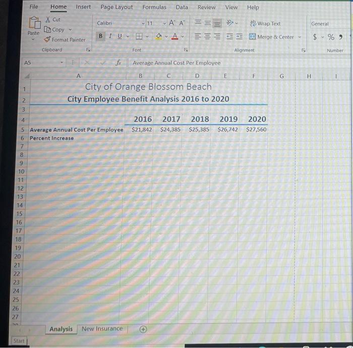
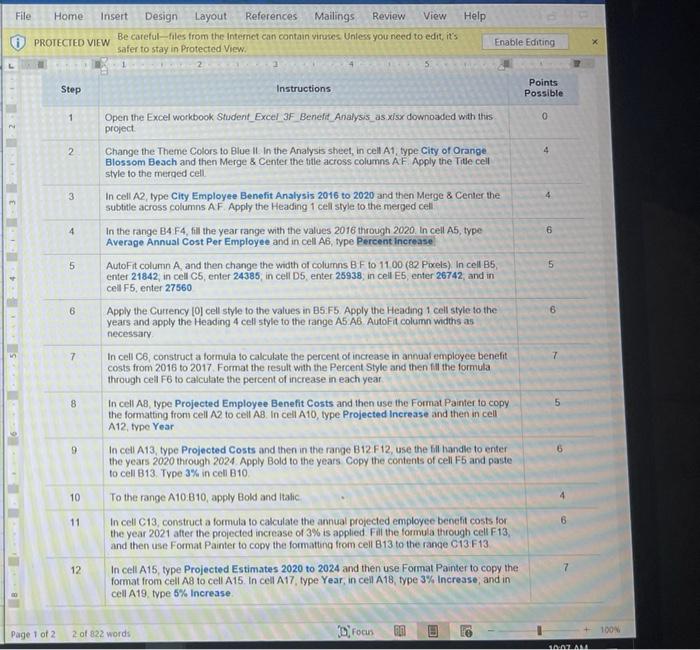
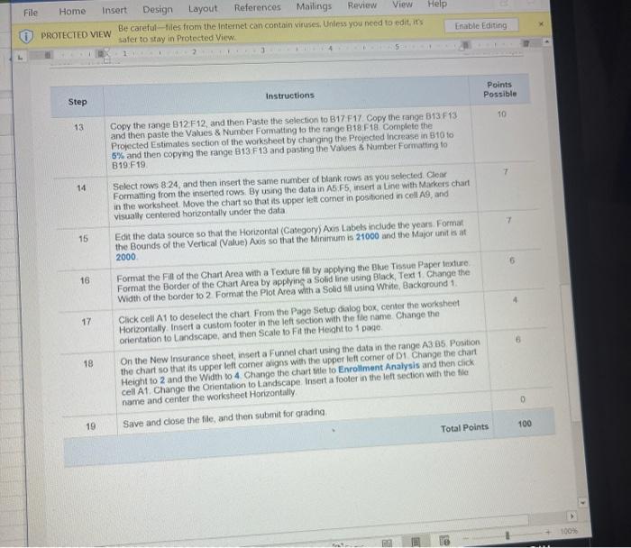
File Home Insert Page Layout Formulas Data Review View Help 2 Wrap Text General x cut [b Copy ~ Format Painter Calibri 11 AA BIU A Paste = == Merge & Center $ %) Clipboard Font Alignment Number AS F G H Average Annual Cost Per Employee A B C D E City of Orange Blossom Beach City Employee Benefit Analysis 2016 to 2020 1 2 3 2018 2019 2020 $25,385 $26,742 $27,560 4 2016 2017 5 Average Annual Cost Per Employee $21,842 $24,385 6 Percent Increase 7 8 9 10 11 12 13 14 15 16 17 18 19 20 21 22 23 24 25 26 27 Analysis New Insurance Start View Help File Home Insert Design Layout References Mailings Review Be careful-files from the Internet can contain viruses. Unless you need to edit. it's PROTECTED VIEW safer to stay in Protected View Enable Editing Step Instructions Points Possible 1 0 2 4 3 4 E 6 5 5 6 6 7 Open the Excel workbook Student Excel 3F_Benefit Analysis as xis: downoaded with this project Change the Theme Colors to Blue it in the Analysis sheet, in cell A1, type City of Orange Blossom Beach and then Merge & Center the title across columns AF Apply the Title cell style to the merged cell In cell A2 type City Employee Benefit Analysis 2016 to 2020 and then Merge & Center the subtitle across columns AF Apply the Heading 1 cell style to the merged cell In the range B4 F4, fill the year range with the values 2016 through 2020. In cell A5, type Average Annual Cost Per Employee and in cell A6, type Percent increase AutoFit column A and then change the width of columns B F to 11 00 (82 Pixels) In cell B5 enter 21842, in cell C5, enter 24385, in cell D5 enter 26938, in cell E5, enter 26742, and in cell F5, enter 27560 Apply the Currency [0cell style to the values in B5:F5. Apply the Heading 1 cell style to the years and apply the Heading 4 cell style to the range A5 A6 AutoFit column widths as necessary In cell C6, construct a formula to calculate the percent of increase in annual employee benefit costs from 2016 to 2017 Format the result with the Percent Style and then fill the formula through cell F6 to calculate the percent of increase in each year In cell A8, type Projected Employee Benefit Costs and then use the Format Painter to copy the formatting from cell A2 to cell A8In cell A10, type Projected Increase and then in cell A12 type Year In cell A13, type Projected Costs and then in the range B12 F12, use the file handle to enter the years 2020 through 2024 Apply Bold to the years Copy the contents of cell F5 and paste to cell B13 Type 3% in cell 810 To the range A10:110, apply Bold and Italic In cell C13, construct a formula to calculate the annual projected employee benefit costs for the year 2021 after the projected increase of 3% is applied Fill the formula through cell F13, and then use Format Painter to copy the formatting from cell B13 to the range C13 F13 In cell A15, type Projected Estimates 2020 to 2024 and then use Format Painter to copy the format from cell As to cell A15. In cell A17 type Year, in cell A18 type 3% Increase, and in cell A19 type 5% Increase 7 8 5 9 10 11 6 12 7 Page 1 of 2 2 of 822 words Droon 100N CIAALANL Help File Home Insert Design Layout References Mailings Review View Be careful-files from the Internet can contain Viruses. Unless you need to edit its PROTECTED VIEW safer to stay in Protected View 2 3 Enable Editing ! Points Possible Instructions Step 10 13 Copy the range B12 F12, and then Paste the selection to B17 F17 Copy the range B13 F13 and then paste the Values & Number Formatting to the range B18 F18. Complete the Projected Estimates section of the worksheet by changing the Projected increase in B10 to 6% and then copying the range 313 F13 and pasting the values & Number Formatting to B19:19 7 14 Select rows 8.24, and then insert the same number of blank rows as you selected. Clear Formatting from the inserted rows. By using the data in A5 F5, insert a Live with Markers chart in the worksheet Move the chart so that its upper left corner in positioned in cell A9, and visually centered horizontally under the data Edit the data source so that the Horizontal (Category) Axis Labels include the years Format the Bounds of the Vertical (Value) Acis so that the Minimum is 21000 and the Major unit is at 2000 7 15 16 17 Format the Fill of the Chart Area with a Texture fil by applying the Blue Tissue Paper fexture Format the Border of the Chart Area by applying a Solid line using Black, Text 1 Change the Width of the border 10 2 Format the Plot Area with a solid fill using White Background 1 Click cell A1 to deselect the chart From the Page Setup dialog box, center the worksheet Horizontally. Insor a custom footer in the left section with the file name Change the orientation to Landscape, and then Scale to Fa the Height to 1 page On the New Insurance sheet, insert a Funnel chart using the data in the range A3 85. Position the chart so that its upper left corner aligns with the upper left comer of D1 Change the chart Height to 2 and the Width to 4 Change the chart title to Enrollment Analysis and then click cell A1 Change the Orientation to Landscape Insert a footer in the left section with the file name and center the worksheet Horizontally Save and close the file, and then submit for grading 18 19 100 Total Points 100% File Home Insert Page Layout Formulas Data Review View Help 2 Wrap Text General x cut [b Copy ~ Format Painter Calibri 11 AA BIU A Paste = == Merge & Center $ %) Clipboard Font Alignment Number AS F G H Average Annual Cost Per Employee A B C D E City of Orange Blossom Beach City Employee Benefit Analysis 2016 to 2020 1 2 3 2018 2019 2020 $25,385 $26,742 $27,560 4 2016 2017 5 Average Annual Cost Per Employee $21,842 $24,385 6 Percent Increase 7 8 9 10 11 12 13 14 15 16 17 18 19 20 21 22 23 24 25 26 27 Analysis New Insurance Start View Help File Home Insert Design Layout References Mailings Review Be careful-files from the Internet can contain viruses. Unless you need to edit. it's PROTECTED VIEW safer to stay in Protected View Enable Editing Step Instructions Points Possible 1 0 2 4 3 4 E 6 5 5 6 6 7 Open the Excel workbook Student Excel 3F_Benefit Analysis as xis: downoaded with this project Change the Theme Colors to Blue it in the Analysis sheet, in cell A1, type City of Orange Blossom Beach and then Merge & Center the title across columns AF Apply the Title cell style to the merged cell In cell A2 type City Employee Benefit Analysis 2016 to 2020 and then Merge & Center the subtitle across columns AF Apply the Heading 1 cell style to the merged cell In the range B4 F4, fill the year range with the values 2016 through 2020. In cell A5, type Average Annual Cost Per Employee and in cell A6, type Percent increase AutoFit column A and then change the width of columns B F to 11 00 (82 Pixels) In cell B5 enter 21842, in cell C5, enter 24385, in cell D5 enter 26938, in cell E5, enter 26742, and in cell F5, enter 27560 Apply the Currency [0cell style to the values in B5:F5. Apply the Heading 1 cell style to the years and apply the Heading 4 cell style to the range A5 A6 AutoFit column widths as necessary In cell C6, construct a formula to calculate the percent of increase in annual employee benefit costs from 2016 to 2017 Format the result with the Percent Style and then fill the formula through cell F6 to calculate the percent of increase in each year In cell A8, type Projected Employee Benefit Costs and then use the Format Painter to copy the formatting from cell A2 to cell A8In cell A10, type Projected Increase and then in cell A12 type Year In cell A13, type Projected Costs and then in the range B12 F12, use the file handle to enter the years 2020 through 2024 Apply Bold to the years Copy the contents of cell F5 and paste to cell B13 Type 3% in cell 810 To the range A10:110, apply Bold and Italic In cell C13, construct a formula to calculate the annual projected employee benefit costs for the year 2021 after the projected increase of 3% is applied Fill the formula through cell F13, and then use Format Painter to copy the formatting from cell B13 to the range C13 F13 In cell A15, type Projected Estimates 2020 to 2024 and then use Format Painter to copy the format from cell As to cell A15. In cell A17 type Year, in cell A18 type 3% Increase, and in cell A19 type 5% Increase 7 8 5 9 10 11 6 12 7 Page 1 of 2 2 of 822 words Droon 100N CIAALANL Help File Home Insert Design Layout References Mailings Review View Be careful-files from the Internet can contain Viruses. Unless you need to edit its PROTECTED VIEW safer to stay in Protected View 2 3 Enable Editing ! Points Possible Instructions Step 10 13 Copy the range B12 F12, and then Paste the selection to B17 F17 Copy the range B13 F13 and then paste the Values & Number Formatting to the range B18 F18. Complete the Projected Estimates section of the worksheet by changing the Projected increase in B10 to 6% and then copying the range 313 F13 and pasting the values & Number Formatting to B19:19 7 14 Select rows 8.24, and then insert the same number of blank rows as you selected. Clear Formatting from the inserted rows. By using the data in A5 F5, insert a Live with Markers chart in the worksheet Move the chart so that its upper left corner in positioned in cell A9, and visually centered horizontally under the data Edit the data source so that the Horizontal (Category) Axis Labels include the years Format the Bounds of the Vertical (Value) Acis so that the Minimum is 21000 and the Major unit is at 2000 7 15 16 17 Format the Fill of the Chart Area with a Texture fil by applying the Blue Tissue Paper fexture Format the Border of the Chart Area by applying a Solid line using Black, Text 1 Change the Width of the border 10 2 Format the Plot Area with a solid fill using White Background 1 Click cell A1 to deselect the chart From the Page Setup dialog box, center the worksheet Horizontally. Insor a custom footer in the left section with the file name Change the orientation to Landscape, and then Scale to Fa the Height to 1 page On the New Insurance sheet, insert a Funnel chart using the data in the range A3 85. Position the chart so that its upper left corner aligns with the upper left comer of D1 Change the chart Height to 2 and the Width to 4 Change the chart title to Enrollment Analysis and then click cell A1 Change the Orientation to Landscape Insert a footer in the left section with the file name and center the worksheet Horizontally Save and close the file, and then submit for grading 18 19 100 Total Points 100%