%% Finite Difference (FD) computation loop

% Important: Other parameters may not be mentioned here,

% and you might need to define them.

xm = 80; %km

dx = 1; %km

dt = 0.2; %s

B = 2; %km/s

sd = 4; %s

sp = 60; %km

tmax = 8; %s

U_0 = zeros(xm/dx,1); %previous i-1

U_1 = zeros(xm/dx,1); %current i

U_2 = zeros(xm/dx,1); %future i+1

nsp = sp/dx; % this is where the source will be positioned

for j=0:round(tmax/dt+1)

t = dt*j;

% Calculate U2 based on U1 and U0, see equation (7)

% Note that the t terms are not explicitly used in this part

for i=2:nx-1

U_2(i) = (B*dt/dx)^2*()

end

%% Boundary conditions

U_2(1) = 0.0; % Left side of grid

U_2(nx) = 0.0; % Right side of grid

%% Source function , see equation (8)

if t

U_2(nsp) = 1.0 - cos(2*pi*t/sd);

end

%% Loop to set current displacement value to past displacement value

% and future displacement value to current displacement value. This is

% where the t aspect of equation 7 comes in.

for i=1:nx

U_0(i) = U_1(i);

U_1(i) = U_2(i);

end

%% Plots for each time step should be here

% ~~~Complete me!~~~

end

%% Plots to be saved should be here

% ~~~Complete me!~~~

%% Save the needed data to be used in the next program!

% ~~~Complete me!~~~

****Could you please just do the complete me sections of this code? question 2a-3 to help me better understand what is happening?

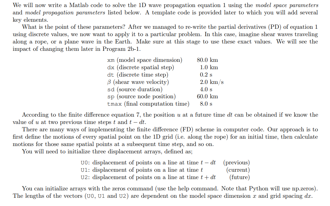
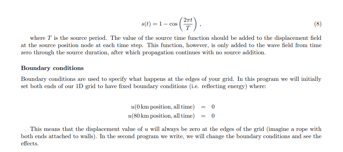
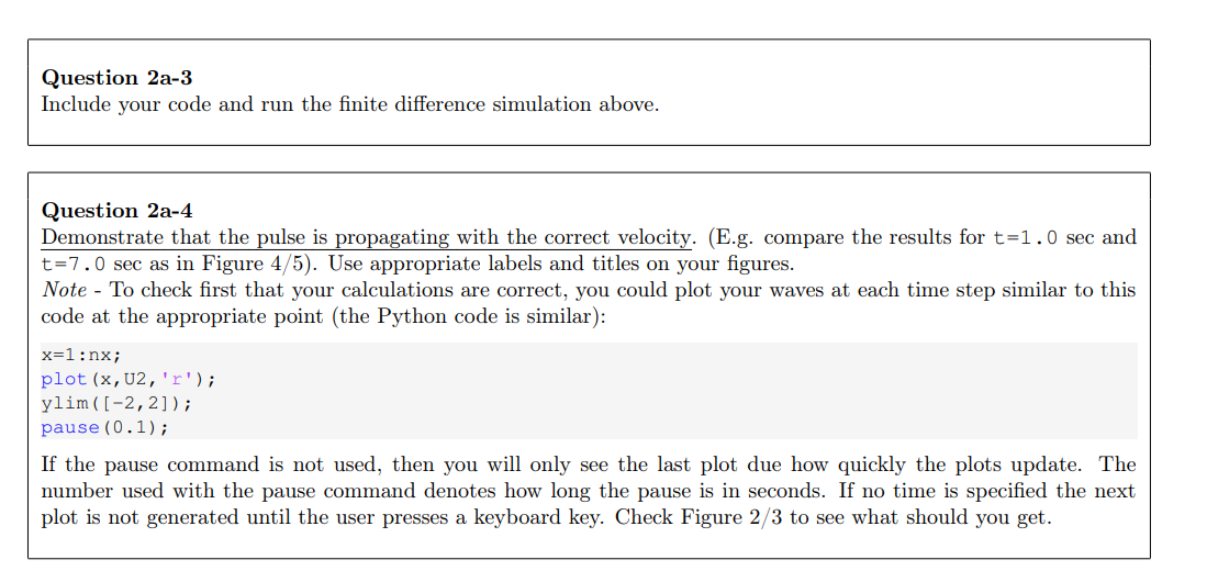
We will now write a Matlab code to solve the 1D wave propagation equation 1 using the model space parameters and model propagation parameters listed below. A template code is provided later to which you will add several key elements. What is the point of these parameters? After we managed to re-write the partial derivatives (PD) of equation 1 using discrete values, we now want to apply it to a particular problem. In this case, imagine shear waves traveling along a rope, or a plane wave in the Earth. Make sure at this stage to use these exact values. We will see the impact of changing them later in Program 2b-1. According to the finite difference equation 7 , the position u at a future time dt can be obtained if we know the value of u at two previous time steps t and tdt. There are many ways of implementing the finite difference (FD) scheme in computer code. Our approach is to first define the motions of every spatial point on the 1D grid (i.e. along the rope) for an initial time, then calculate motions for those same spatial points at a subsequent time step, and so on. You will need to initialize three displacement arrays, defined as; U0:displacementofpointsonalineattimetdtU1:displacementofpointsonalineattimetU2:displacementofpointsonalineattimet+dt(previous)(current)(future) You can initialize arrays with the zeros command (use the help command. Note that Python will use np.zeros). The lengths of the vectors (U0, U1 and U2) are dependent on the model space dimension x and grid spacing dx. s(t)=1cos(T2t) where T is the source period. The value of the source time function should be added to the displacement field at the source position node at each time step. This function, however, is only added to the wave field from time zero through the source duration, after which propagation continues with no source addition. Boundary conditions Boundary conditions are used to specify what happens at the edges of your grid. In this program we will initially set both ends of our 1D grid to have fixed boundary conditions (i.e. reflecting energy) where: u(0kmposition,alltime)u(80kmposition,alltime)=0=0 This means that the displacement value of u will always be zero at the edges of the grid (imagine a rope with both ends attached to walls). In the second program we write, we will change the boundary conditions and see the effects. Question 2a-3 Include your code and run the finite difference simulation above. Question 2a-4 Demonstrate that the pulse is propagating with the correct velocity. (E.g. compare the results for t=1.0 sec and t=7.0 sec as in Figure 4/5). Use appropriate labels and titles on your figures. Note - To check first that your calculations are correct, you could plot your waves at each time step similar to this code at the appropriate point (the Python code is similar): x=1:nx; plot (x,U2,x); ylim([2,2]); pause (0.1); If the pause command is not used, then you will only see the last plot due how quickly the plots update. The number used with the pause command denotes how long the pause is in seconds. If no time is specified the next plot is not generated until the user presses a keyboard key. Check Figure 2/3 to see what should you get