Formulas: Insert three columns after the Product Cost. Title the first column: Shipping Costs. Title the second column: Order Total Cost and title the third column: Projected Revenue. Insert a column at the end of the data. Title that column: Days in Transit. Create a formula for the Product Cost. It is derived by multiplying Item Cost by Quantity. Create a formula for the Shipping Costs. Shipping costs are made up of two components a base shipping charge plus a shipping rate times the product cost. Both of those values are given on the worksheet titled Inputs. The formula for the Shipping Costs column must reference the cell addresses on the Inputs worksheet and use absolute cell addressing. Also pay attention to the order of math operations in your formula. Create a formula for the Order Total Cost. It is derived by adding the Product Cost and the Shipping Costs. Create a formula for the Projected Revenue. It is calculated by multiplying the Product Cost times the Standard Product Markup given on the worksheet titled Inputs Create a formula for the Days in Transit by subtracting the Ship Date from the Arrival Date. Be sure that the result is reflected in days. Add totals at the bottom of the spreadsheet for the appropriate columns. Presentation: Insert rows at the top of the worksheet and create a formatted and centered page title: ABC Company Order & Shipping Report Format each of the columns of data in the worksheet to wrap the column headings. Ensure that the contents of the cells are visible and offset the column headings with some shading and/or cell borders. Sort the data by Vendor Name and Item# Apply all necessary formatting to the data to display it in a meaningful way (alignment, number and date formatting, column width, etc). Insert a custom page footer to print page numbers on the bottom right and the file path and name at the bottom left of each page. Force the document to print all the columns on a single page in Landscape mode. It should span two pages in length but all columns must appear on a single page. In case the printed document spans more than one page vertically set the top column headings to reprint on each subsequent page.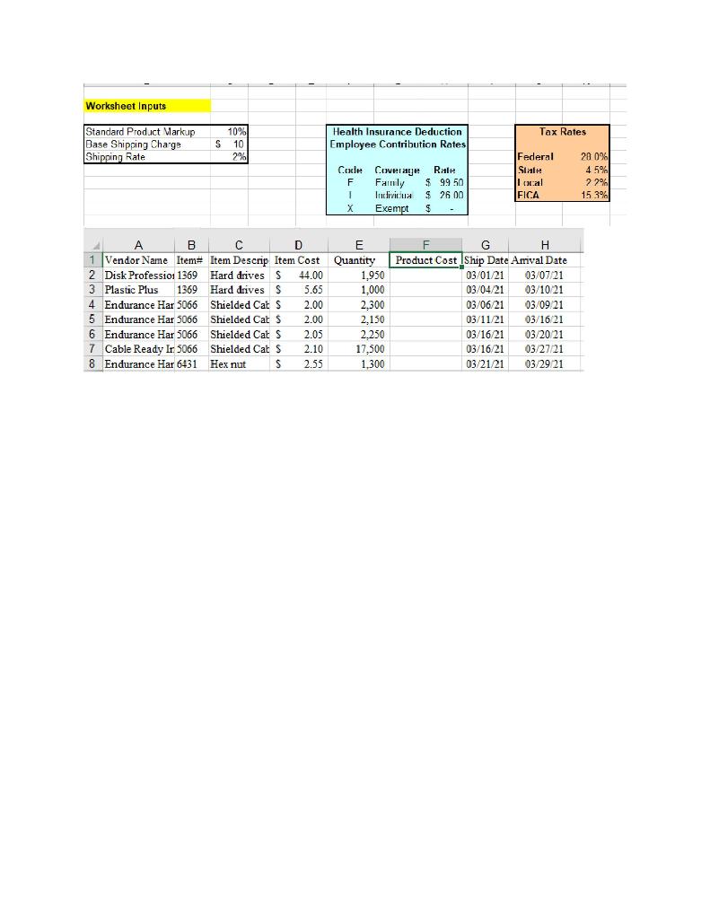

Worksheet Inputs Standard Product Markup Base Shipping Charge Shipping Rate A B 4 1 Vendor Name Item# 2 Disk Profession 1369 3 Plastic Plus 1369 Endurance Har 5066 5 Endurance Har 5066 6 Endurance Har 5066 7 Cable Ready Ir 5066 8 Endurance Har 6431 10% 10 2% C D Item Descrip Item Cost Hard drives S 44.00 Hard drives S 5.65 Shielded Cat S 2.00 Shielded Cat S Shielded Cat S Shielded Cat S Hex nut 2,00 2.05 2.10 S 2.55 S Health Insurance Deduction Employee Contribution Rates Federal State Code Coverage Rale Family F $ 99 50 local Individua $26.00 FICA Exempt $ F G H Product Cost Ship Date Arrival Date 03/01/21 03/07/21 03/04/21 03/10/21 03/06/21 03/09/21 03/11/21 03/16/21 03/16/21 03/20/21 03/16/21 03/27/21 03/21/21 03/29/21 T X E Quantity 1,950 1,000 2.300 2,150 2.250 17,500 1,300 Tax Rates. 20 0% 4 5% 22% 15.3%