give detailed conclusions

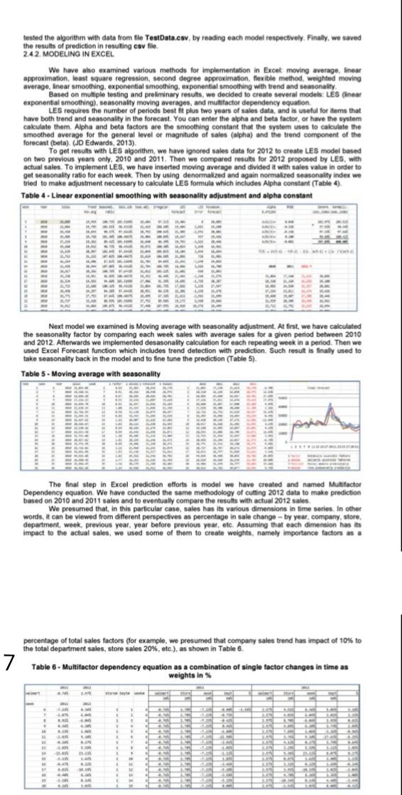
tested the algorithm with data from file TestData.csv by reading each model respectively. Finally, we saved , . the results of prediction in resulting csv file 242. MODELING IN EXCEL We have also examined various methods for implementation in Excel moving average, linear approximation, least square regression second degree approximation, flexible method. weighted moving averago, linear smoothing, exponential smoothing, exponential smoothing with trend and seasonality Based on multiple testing and preliminary results, we decided to create several models: LES Oinear exponential smoothing), seasonality moving averages, and multifactor dependency equation LES requires the number of periods best fit plus two years of sales data, and is useful for items that have both trend and seasonality in the forecast. You can enter the alpha and beta factor, or have the system calculate them. Alpha and beta factors are the smoothing constant that the system uses to calculate the smoothed average for the general level or magnitude of sales (alpha) and the trend component of the forecast (beta) (JD Edwards, 2013) To get results with LES algorithm, we have ignored sales data for 2012 to create LES model based on two previous years only, 2010 and 2011. Then we compared results for 2012 proposed by LES, with actual sales. To implement LES, we have inserted moving average and divided it with sales value in order to get seasonality ratio for each week. Then by using denormalized and again normalized seasonality index we tried to make adjustment necessary to calculate LES formula which includes Alpha constant (Table 4). Table 4 - Linear exponential smoothing with seasonality adjustment and alpha constant - Next model we examined is Moving average with seasonality adjustment. At first, we have calculated the seasonality factor by comparing each week sales with average sales for a given period between 2010 and 2012. Afterwards we implemented desasonality calculation for each repeating week in a period. Then we used Excel Forecast function which includes trend detection with prediction. Such result is finally used to take seasonality back in the model and to fine tune the prediction (Table 5). Table 5. Moving average with seasonality 5 The final step in Excel prediction efforts is model we have created and named Multifactor Dependency equation. We have conducted the same methodology of cutting 2012 data to make prediction based on 2010 and 2011 sales and to eventually compare the results with actual 2012 sales We presumed that in this particular case, sales has its various dimensions in time series. In other words, it can be viewed from different perspectives as percentage in sale change - by year, company, store, department, week. previous year, year before previous year, etc. Assuming that each dimension has its Impact to the actual sales, we used some of them to create weights, namely importance factors as a percentage of total sales factors (for example, we presumed that company sales trend has impact of 10% to the total department sales, store sales 20%, etc.), as shown in Table 6. 7 Table 6 - Multifactor dependency equation as a combination of single factor changes in time as weights in . . AM m