

Go Sports Anton Aliyev is the store manager for Go Sports, a sports clothing store in...
Fantastic news! We've Found the answer you've been seeking!
Question:
Transcribed Image Text:
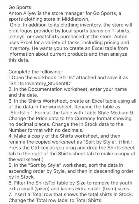
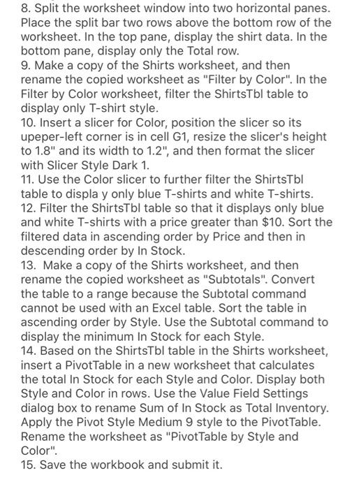
Go Sports Anton Aliyev is the store manager for Go Sports, a sports clothing store in Middletown, Ohio. In addition to its clothing inventory, the store will print logos provided by local sports teams on T-shirts, jerseys, or sweatshirts purchased at the store. Anton uses Excel for a variety of tasks, including pricing and inventory. He wants you to create an Excel table from information about current products and then analyze this data. Complete the following: 1.0pen the workbook "Shirts" attached and save it as "Shirts Inventory_StudentID" 2. In the Documentation worksheet, enter your name and the date. 3. In the Shirts Worksheet, create an Excel table using all of the data in the worksheet. Rename the table as "ShirtsTbl". Format the table with Table Style Medium 9. Change the Price data to the Currency format showing no decimal places. Change the In Stock data to the Number format with no decimals. 4. Make a cop y of the Shirts worksheet, and then rename the copied worksheet as "Sort by Style". (Hint : Press the Ctrl key as you drag and drop the Shirts sheet tab to the right of the Shirts sheet tab to make a copy of the worksheet.) 5. In the "Sort by Style" worksheet, sort the data in ascending order by Style, and then in descending order by In Stock. 6. Filter the ShirtsTbl table by Size to remove the youth extra small (yxsm) and ladies extra small (Ixsm) sizes. 7. Insert a Total row that shows the total shirts In Stock. Change the Total row label to Total Shirts. 8. Split the worksheet window into two horizontal panes. Place the split bar two rows above the bottom row of the worksheet. In the top pane, display the shirt data. In the bottom pane, display only the Total row. 9. Make a copy of the Shirts worksheet, and then rename the copied worksheet as "Filter by Color". In the Filter by Color worksheet, filter the ShirtsTbl table to display only T-shirt style. 10. Insert a slicer for Color, position the slicer so its upeper-left corner is in cell G1, resize the slicer's height to 1.8" and its width to 1.2", and then format the slicer with Slicer Style Dark 1. 11. Use the Color slicer to further filter the ShirtsTbl table to displa y only blue T-shirts and white T-shirts. 12. Filter the ShirtsTbl table so that it displays only blue and white T-shirts with a price greater than $10. Sort the filtered data in ascending order by Price and then in descending order by In Stock. 13. Make a copy of the Shirts worksheet, and then rename the copied worksheet as "Subtotals". Convert the table to a range because the Subtotal command cannot be used with an Excel table. Sort the table in ascending order by Style. Use the Subtotal command to display the minimum In Stock for each Style. 14. Based on the ShirtsTbl table in the Shirts worksheet, insert a PivotTable in a new worksheet that calculates the total In Stock for each Style and Color. Display both Style and Color in rows. Use the Value Field Settings dialog box to rename Sum of In Stock as Total Inventory. Apply the Pivot Style Medium 9 style to the PivotTable. Rename the worksheet as "PivotTable by Style and Color". 15. Save the workbook and submit it. Go Sports Anton Aliyev is the store manager for Go Sports, a sports clothing store in Middletown, Ohio. In addition to its clothing inventory, the store will print logos provided by local sports teams on T-shirts, jerseys, or sweatshirts purchased at the store. Anton uses Excel for a variety of tasks, including pricing and inventory. He wants you to create an Excel table from information about current products and then analyze this data. Complete the following: 1.0pen the workbook "Shirts" attached and save it as "Shirts Inventory_StudentID" 2. In the Documentation worksheet, enter your name and the date. 3. In the Shirts Worksheet, create an Excel table using all of the data in the worksheet. Rename the table as "ShirtsTbl". Format the table with Table Style Medium 9. Change the Price data to the Currency format showing no decimal places. Change the In Stock data to the Number format with no decimals. 4. Make a cop y of the Shirts worksheet, and then rename the copied worksheet as "Sort by Style". (Hint : Press the Ctrl key as you drag and drop the Shirts sheet tab to the right of the Shirts sheet tab to make a copy of the worksheet.) 5. In the "Sort by Style" worksheet, sort the data in ascending order by Style, and then in descending order by In Stock. 6. Filter the ShirtsTbl table by Size to remove the youth extra small (yxsm) and ladies extra small (Ixsm) sizes. 7. Insert a Total row that shows the total shirts In Stock. Change the Total row label to Total Shirts. 8. Split the worksheet window into two horizontal panes. Place the split bar two rows above the bottom row of the worksheet. In the top pane, display the shirt data. In the bottom pane, display only the Total row. 9. Make a copy of the Shirts worksheet, and then rename the copied worksheet as "Filter by Color". In the Filter by Color worksheet, filter the ShirtsTbl table to display only T-shirt style. 10. Insert a slicer for Color, position the slicer so its upeper-left corner is in cell G1, resize the slicer's height to 1.8" and its width to 1.2", and then format the slicer with Slicer Style Dark 1. 11. Use the Color slicer to further filter the ShirtsTbl table to displa y only blue T-shirts and white T-shirts. 12. Filter the ShirtsTbl table so that it displays only blue and white T-shirts with a price greater than $10. Sort the filtered data in ascending order by Price and then in descending order by In Stock. 13. Make a copy of the Shirts worksheet, and then rename the copied worksheet as "Subtotals". Convert the table to a range because the Subtotal command cannot be used with an Excel table. Sort the table in ascending order by Style. Use the Subtotal command to display the minimum In Stock for each Style. 14. Based on the ShirtsTbl table in the Shirts worksheet, insert a PivotTable in a new worksheet that calculates the total In Stock for each Style and Color. Display both Style and Color in rows. Use the Value Field Settings dialog box to rename Sum of In Stock as Total Inventory. Apply the Pivot Style Medium 9 style to the PivotTable. Rename the worksheet as "PivotTable by Style and Color". 15. Save the workbook and submit it. Go Sports Anton Aliyev is the store manager for Go Sports, a sports clothing store in Middletown, Ohio. In addition to its clothing inventory, the store will print logos provided by local sports teams on T-shirts, jerseys, or sweatshirts purchased at the store. Anton uses Excel for a variety of tasks, including pricing and inventory. He wants you to create an Excel table from information about current products and then analyze this data. Complete the following: 1.0pen the workbook "Shirts" attached and save it as "Shirts Inventory_StudentID" 2. In the Documentation worksheet, enter your name and the date. 3. In the Shirts Worksheet, create an Excel table using all of the data in the worksheet. Rename the table as "ShirtsTbl". Format the table with Table Style Medium 9. Change the Price data to the Currency format showing no decimal places. Change the In Stock data to the Number format with no decimals. 4. Make a cop y of the Shirts worksheet, and then rename the copied worksheet as "Sort by Style". (Hint : Press the Ctrl key as you drag and drop the Shirts sheet tab to the right of the Shirts sheet tab to make a copy of the worksheet.) 5. In the "Sort by Style" worksheet, sort the data in ascending order by Style, and then in descending order by In Stock. 6. Filter the ShirtsTbl table by Size to remove the youth extra small (yxsm) and ladies extra small (Ixsm) sizes. 7. Insert a Total row that shows the total shirts In Stock. Change the Total row label to Total Shirts. 8. Split the worksheet window into two horizontal panes. Place the split bar two rows above the bottom row of the worksheet. In the top pane, display the shirt data. In the bottom pane, display only the Total row. 9. Make a copy of the Shirts worksheet, and then rename the copied worksheet as "Filter by Color". In the Filter by Color worksheet, filter the ShirtsTbl table to display only T-shirt style. 10. Insert a slicer for Color, position the slicer so its upeper-left corner is in cell G1, resize the slicer's height to 1.8" and its width to 1.2", and then format the slicer with Slicer Style Dark 1. 11. Use the Color slicer to further filter the ShirtsTbl table to displa y only blue T-shirts and white T-shirts. 12. Filter the ShirtsTbl table so that it displays only blue and white T-shirts with a price greater than $10. Sort the filtered data in ascending order by Price and then in descending order by In Stock. 13. Make a copy of the Shirts worksheet, and then rename the copied worksheet as "Subtotals". Convert the table to a range because the Subtotal command cannot be used with an Excel table. Sort the table in ascending order by Style. Use the Subtotal command to display the minimum In Stock for each Style. 14. Based on the ShirtsTbl table in the Shirts worksheet, insert a PivotTable in a new worksheet that calculates the total In Stock for each Style and Color. Display both Style and Color in rows. Use the Value Field Settings dialog box to rename Sum of In Stock as Total Inventory. Apply the Pivot Style Medium 9 style to the PivotTable. Rename the worksheet as "PivotTable by Style and Color". 15. Save the workbook and submit it. Go Sports Anton Aliyev is the store manager for Go Sports, a sports clothing store in Middletown, Ohio. In addition to its clothing inventory, the store will print logos provided by local sports teams on T-shirts, jerseys, or sweatshirts purchased at the store. Anton uses Excel for a variety of tasks, including pricing and inventory. He wants you to create an Excel table from information about current products and then analyze this data. Complete the following: 1.0pen the workbook "Shirts" attached and save it as "Shirts Inventory_StudentID" 2. In the Documentation worksheet, enter your name and the date. 3. In the Shirts Worksheet, create an Excel table using all of the data in the worksheet. Rename the table as "ShirtsTbl". Format the table with Table Style Medium 9. Change the Price data to the Currency format showing no decimal places. Change the In Stock data to the Number format with no decimals. 4. Make a cop y of the Shirts worksheet, and then rename the copied worksheet as "Sort by Style". (Hint : Press the Ctrl key as you drag and drop the Shirts sheet tab to the right of the Shirts sheet tab to make a copy of the worksheet.) 5. In the "Sort by Style" worksheet, sort the data in ascending order by Style, and then in descending order by In Stock. 6. Filter the ShirtsTbl table by Size to remove the youth extra small (yxsm) and ladies extra small (Ixsm) sizes. 7. Insert a Total row that shows the total shirts In Stock. Change the Total row label to Total Shirts. 8. Split the worksheet window into two horizontal panes. Place the split bar two rows above the bottom row of the worksheet. In the top pane, display the shirt data. In the bottom pane, display only the Total row. 9. Make a copy of the Shirts worksheet, and then rename the copied worksheet as "Filter by Color". In the Filter by Color worksheet, filter the ShirtsTbl table to display only T-shirt style. 10. Insert a slicer for Color, position the slicer so its upeper-left corner is in cell G1, resize the slicer's height to 1.8" and its width to 1.2", and then format the slicer with Slicer Style Dark 1. 11. Use the Color slicer to further filter the ShirtsTbl table to displa y only blue T-shirts and white T-shirts. 12. Filter the ShirtsTbl table so that it displays only blue and white T-shirts with a price greater than $10. Sort the filtered data in ascending order by Price and then in descending order by In Stock. 13. Make a copy of the Shirts worksheet, and then rename the copied worksheet as "Subtotals". Convert the table to a range because the Subtotal command cannot be used with an Excel table. Sort the table in ascending order by Style. Use the Subtotal command to display the minimum In Stock for each Style. 14. Based on the ShirtsTbl table in the Shirts worksheet, insert a PivotTable in a new worksheet that calculates the total In Stock for each Style and Color. Display both Style and Color in rows. Use the Value Field Settings dialog box to rename Sum of In Stock as Total Inventory. Apply the Pivot Style Medium 9 style to the PivotTable. Rename the worksheet as "PivotTable by Style and Color". 15. Save the workbook and submit it.
Expert Answer:
Answer rating: 100% (QA)
Step 1 of 29 A Step 1 Open Shirts workbook from data files Save the workbook as Shirts Inventory Shi... View the full answer

Related Book For 

Retail Management A Strategic Approach
ISBN: 978-0132720823
12th edition
Authors: Barry R. Berman, Joel R. Evans
Posted Date:
Students also viewed these general management questions
-
The sales manager at Lorenzo Markets wants you to create an application that displays the total sales made in each of three regions: the U.S., Canada, and Mexico. The application should also display...
-
Mr. Small, the store manager for Jay's Appliance, is having a difficult time placing a selling price on a refrigerator that cost $410. Mr. Small knows his boss would like to have a 45% markup based...
-
K & L Clothiers wants you to create an application that prints a customers sales receipt. A sample receipt is shown in Figure 3-49. Use the following names for the solution and project, respectively:...
-
The Trial Balance and Adjustments columns of the worksheet of Wells Decorating Centre included these accounts and balances at December 31, 2017: Required Wells Decorating Centre uses the perpetual...
-
The following state transition table is a simplified model of process management, with the labels representing transitions between states of READY, RUN, BLOCKED, and NONRESIDENT. Give an example of...
-
Kenneth Wheeler was angry at certain police officers in Grand Junction, Colorado, because of a driving-under-the-influence arrest that he viewed as unjust. While in Italy, Wheeler posted a statement...
-
For each of the following situations, calculate a \(95 \%\) confidence interval for the mean ( \(\sigma\) known), beginning with the step, "Identify the critical value of \(z\)." X = 7.00, o Xe =...
-
On August 1, 2011, Dr. Dana Hendley established Med, a medical practice organized as a professional corporation. The following conversation occurred the following February between Dr. Hendley and a...
-
Frank is usually the first one to arrive at Costco's main warehouse. He primarily builds the work schedules for all the employees in the stock room and manages the performance of the entry-level...
-
It is false that no A are B. Therefore, some A are B. Use the modified Venn diagram technique to determine if the following immediate inference forms are valid from the Boolean standpoint,...
-
Modify your min-heap that stores arbitrary structs Using C language Create 2 files: min_heap.c and min_heap.h To create a min-heap that can sort *any datatype*, we'll utilize void* and function...
-
Cannington Inc. designs, manufactures, and markets personal computers and related software. Cannington also manufactures and distributes music players (cPod), mobile phones (cPhone), and smartwatches...
-
Finch Services Company has 56 employees, 22 of whom are assigned to Division A and 34 to Division B. Finch incurred $347,760 of fringe benefits cost during Year 2. Required Determine the amount of...
-
Dunbar Company had 4 , 0 0 0 , 0 0 0 shares of $ 1 par value common stock outstanding at January 1 , 2 0 2 0 . On July 1 , 2 0 2 0 , the company issued 1 , 0 0 0 , 0 0 0 additional shares of common...
-
BestTech Balance Sheet October 3 1 , 2 0 2 3 Assets Cash $ 4 4 , 0 0 0 Accounts Receivable 7 0 , 5 0 0 Supplies 1 3 , 5 0 0 Land 5 0 , 0 0 0 Total Assets $ 1 7 8 , 0 0 0 Liabilities & Stockholders...
-
Straight-Line, Declining-Balance, and Sum-of-the-Years'-Digits Methods A light truck is purchased on January 1 at a cost of $14,000. It is expected to serve for eight years and have a salvage value...
-
Case Study: ABC Manufacturing Inc. - Accounting for Complex Revenue Recognition Background: ABC Manufacturing Inc. is a global company that specializes in manufacturing high- tech machinery used in...
-
What is the difference between direct materials and indirect materials?
-
Describe the pros and cons of Rue 21 not owning any real-estate.
-
What customer information should Starbucks keep in its retail information system? How could it use this information?
-
Discuss the pros and cons of Coach's "beachhead to a disperse location" strategy.
-
The \(x\) component of the velocity of a car changes from \(-10 \mathrm{~m} / \mathrm{s}\) to \(-2.0 \mathrm{~m} / \mathrm{s}\) in \(10 \mathrm{~s}\). (a) Is the car traveling in the positive or...
-
The day after the incident described in Problem 44, the instructor finds herself in the same situation. This time, she tries a harder physics exercise. She keeps running at a constant \(6.0...
-
(a) A car is speeding up in the negative \(x\) direction. In what direction do \(\vec{a}\) and \(\vec{v}\) point? (b) To which of the four graphs in Figures 3 . 2 and 3 . 3 does the situation...

Study smarter with the SolutionInn App