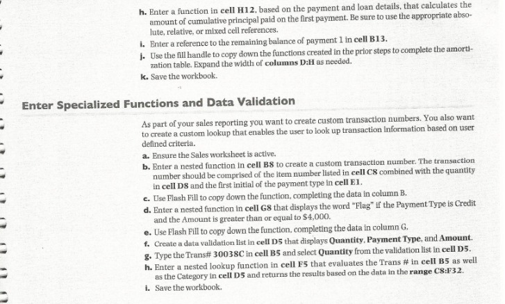
h. Enter a function in cell H12, based on the payment and loan details, that calculates the amount of cumulative principal paid on the first payment. Be sure to use the appropriate abso- lute, relative, or mixed cell references. I. Enter a reference to the remaining balance of payment 1 in cell B13. J. Use the fill handle to copy down the functions created in the prior steps to complete the amorti- zation table. Expand the width of columns D:H as needed. k. Save the workbook. Enter Specialized Functions and Data Validation As part of your sales reporting you want to create custom transaction numbers. You also want to create a custom lookup that enables the user to look up transaction information based on user defined criteria. a. Ensure the Sales worksheet is active. b. Enter a nested function in cell BS to create a custom transaction number. The transaction number should be comprised of the item number listed in cell CS combined with the quantity In cell DS and the first initial of the payment type in cell El. c. Use Flash Fill to copy down the function, completing the data in column B. d. Enter a nested function in cell GS that displays the word "Flag" if the Payment Type is Credit and the Amount is greater than or equal to $4,000. e. Use Flash Fill to copy down the function, completing the data in column G. f. Create a data validation list in cell D5 that displays Quantity, Payment Type, and Amount. g. Type the Trans# 30038C in cell B5 and select Quantity from the validation list in cell DS. h. Enter a nested lookup function in cell F5 that evaluates the Trans # in cell B5 as well as the Category in cell D5 and returns the results based on the data in the range C8:F32. 1. Save the workbook