Hello guys,

can anyone help me with problem 1 and 2?

But they must be computed in Matlab. I am not looking for another type of solution.

Only the codes that I have input in Matlab.Its is to use Anti-derivatives in those functions in Matlab.

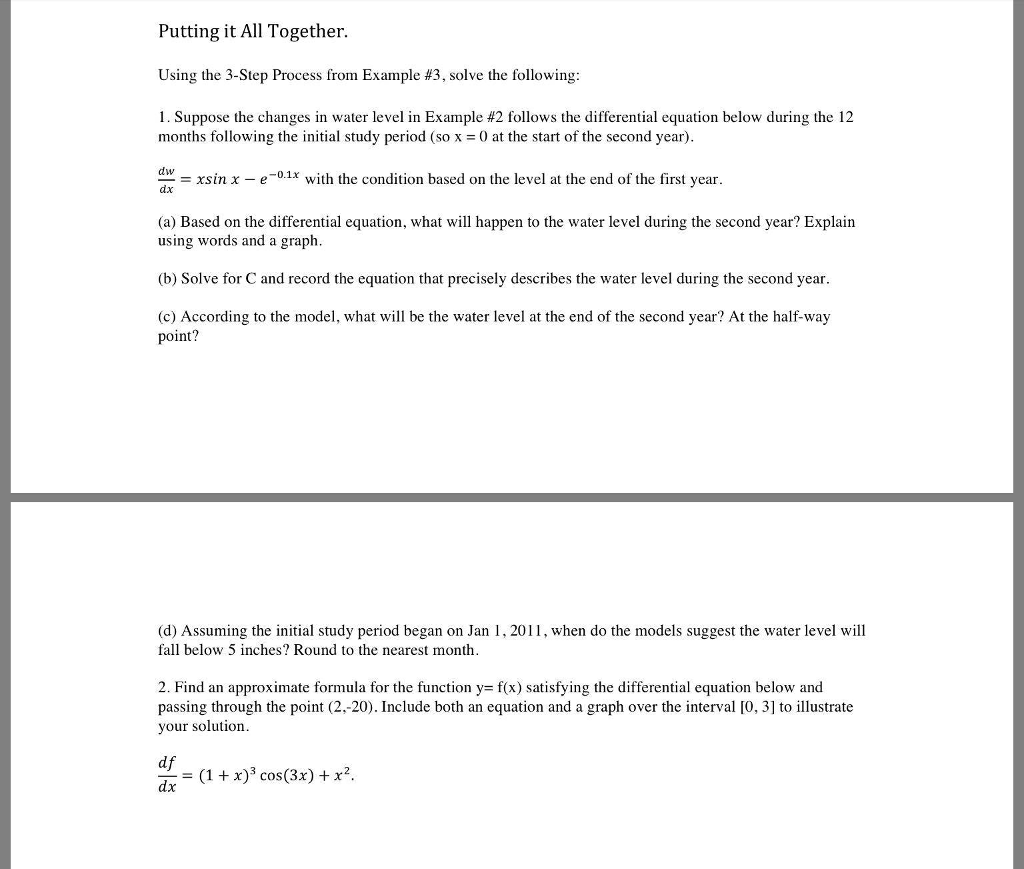
So, I am looking for the codes that I have to write in Mathlab. Please write the explanation of each step. Bellow the images I will show how I did Example 2 and 3 (which respective questions are on image two). So I am looking for similar to question 1 and 2 (which are in the third picture)

Example 2:

>> syms x f(x)

>> f(x)= -9.8*x^2/2+50*x+2;

>> ezplot (f(x),[0,50])

>> grid on

>> vpasolve(f(x),[5,15])

ans =

10.243926050048498207963389797722

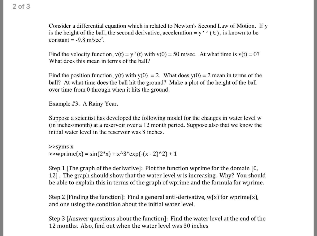
Example 3:

>> syms x

>> wprime(x)=sin(2*x)+x^3*exp(-(x-2)^2)+1;

>> ezplot(wprime(x),[0,12])

>> grid on

>> syms c

>> w(x)= int(wprime(x),x)+c;

>> my_c=solve(w(0)-8,c)

my_c =

(5*exp(-4))/2 + (11*pi^(1/2)*erf(2))/2 + 17/2

>> vpa(my_c)

ans =

18.248684395608473930376586448238

>> w(x)=int(wprime(x),x)+ my_c

w(x) =

x - cos(2*x)/2 + (5*exp(-4))/2 - (5*exp(- x^2 + 4*x - 4))/2 - (x^2*exp(- x^2 + 4*x - 4))/2 + (11*pi^(1/2)*erf(x - 2))/2 + (11*pi^(1/2)*erf(2))/2 - x*exp(- x^2 + 4*x - 4) + 17/2

>> w(0)

ans =

8

>> vpasolve(w(x)-30,x)

ans =

3.5835300620602073995097943314463

>> wprime(x)=sin(2*x)+x^3*exp(-(x-2)^2)+1;

>> syms c

>> w(x)=int(wprime(x),x)+c

w(x) =

c + x - cos(2*x)/2 - (5*exp(- x^2 + 4*x - 4))/2 - (x^2*exp(- x^2 + 4*x - 4))/2 + (11*pi^(1/2)*erf(x - 2))/2 - x*exp(- x^2 + 4*x - 4)

>> my_c=solve(w(0)-8)

my_c =

(5*exp(-4))/2 + (11*pi^(1/2)*erf(2))/2 + 17/2

>> w(x)=int(wprime(x),x)+my_c

w(x) =

x - cos(2*x)/2 + (5*exp(-4))/2 - (5*exp(- x^2 + 4*x - 4))/2 - (x^2*exp(- x^2 + 4*x - 4))/2 + (11*pi^(1/2)*erf(x - 2))/2 + (11*pi^(1/2)*erf(2))/2 - x*exp(- x^2 + 4*x - 4) + 17/2

>> w(0)

ans =

8

>> w(12)

ans =

(5*exp(-4))/2 - cos(24)/2 - (173*exp(-100))/2 + (11*pi^(1/2)*erf(2))/2 + (11*pi^(1/2)*erf(10))/2 + 41/2

>> vpa(ans)

ans =

39.785091071920313592547982134234

>> y=ans

y =

39.785091071920313592547982134234

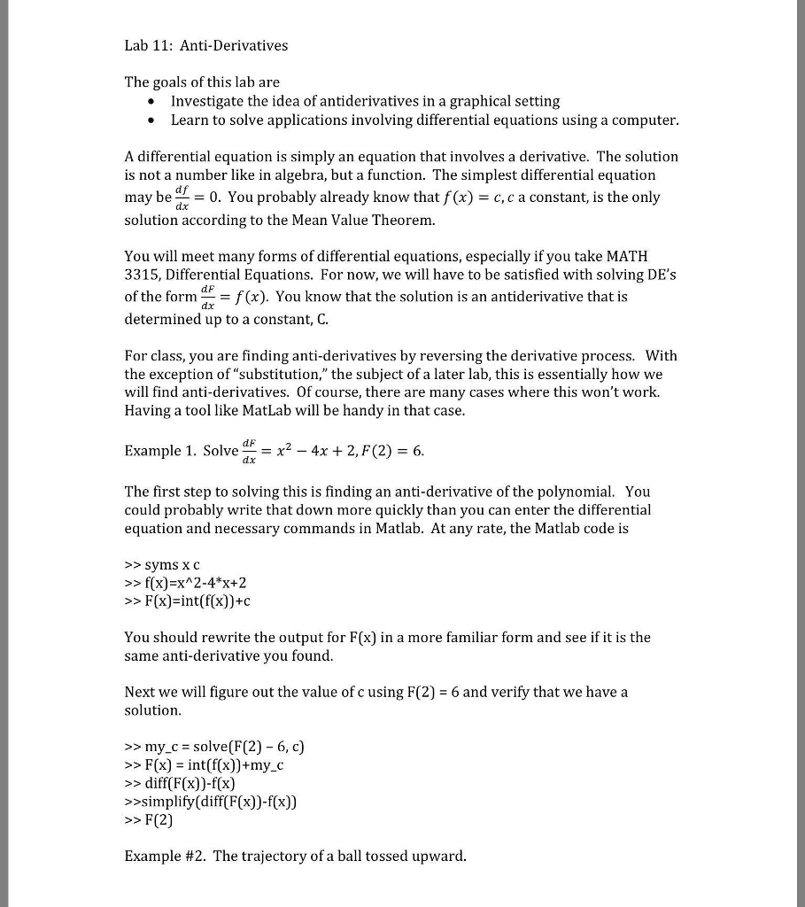
Lab 11: Anti-Derivatives The goals of this lab are Investigate the idea of antiderivatives in a graphical setting Learn to solve applications involving differential equations using a computer. . A differential equation is simply an equation that involves a derivative. The solution is not a number like in algebra, but a function. The simplest differential equation may be -0. You probably already know that f(x) c, c a constant, is the only solution according to the Mean Value Theorem. You will meet many forms of differential equations, especially if you take MATH 3315, Differential Equations. For now, we will have to be satisfied with solving DE's of the form = f(x). You know that the solution is an antiderivative that is determined up to a constant, C. dF For class, you are finding anti-derivatives by reversing the derivative process. With the exception of "substitution," the subject of a later lab, this is essentially how we will find anti-derivatives. Of course, there are many cases where this won't work. Having a tool like MatLab will be handy in that case dF The first step to solving this is finding an anti-derivative of the polynomial. You could probably write that down more quickly than you can enter the differential equation and necessary commands in Matlab. At any rate, the Matlab code is >> syms X C >> f(x)=x^2-4*x+2 >> F(x)=int(f(x))+c You should rewrite the output for F(x) in a more familiar form and see if it is the same anti-derivative you found. Next we will figure out the value of c using F(2) 6 and verify that we have a solution >> my-c = solve(F(2)-6, c) >> F(x) = int(f(x)) +my_c >diff(F(x))-f(x) >>simplify(diff(F(x))-f(x)) Example #2. The trajectory of a ball tossed upward