

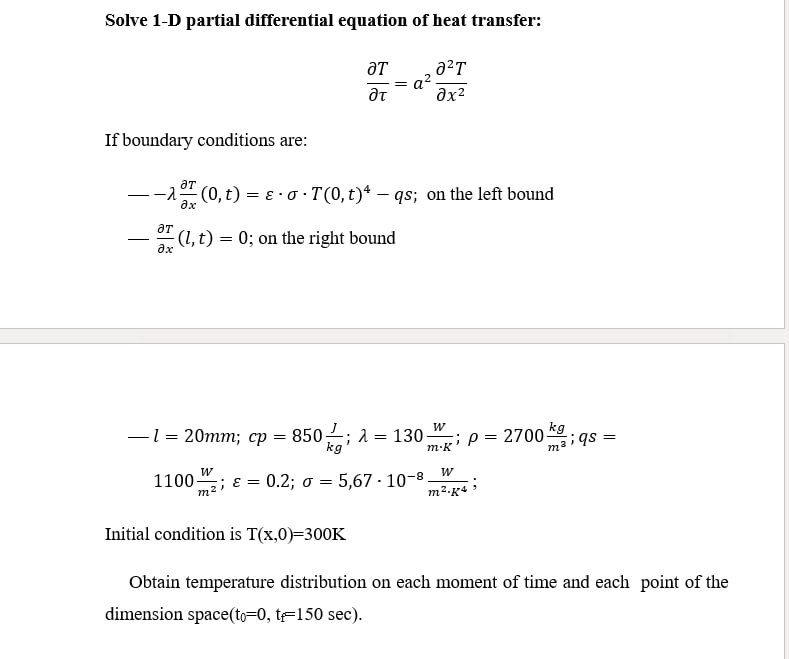
Question: Hello, I ' m doing this problem on 1 - D partial differential equation of heat transfer in math programming class. My code is incorrect
Hello, Im doing this problem on D partial differential equation of heat transfer in math programming class. My code is incorrect because the right boundary question needs to be Neuman's Condition. Please fix my PYTHON code to fit the Neuman Condition and solve the problem. The PYTHON code is below and the picture is the question for which I made the code. import numpy as np
import matplotlib.pyplot as plt
# Parameters
l # Length in meters
cp # Specific heat capacity in JkgK
lambda # Thermal conductivity in WmK
rho # Density in kgm
qs # Heat flux in Wm
epsi # Emissivity
sigma e # StefanBoltzmann constant in WmK
T # Initial temperature in K
# Derived parameters
alpha lambda cp rho # Thermal diffusivity in ms
# Discretization parameters
nx # Number of spatial points
dx l nx # Spatial step size
# Stability criterion for the explicit method
dt dx alpha # Time step size based on stability criterion
nt # Number of time steps
# Initialize temperature array
T nponesnx T
# Function to update temperature distribution
def updatetemperatureT dt dx alpha, lambda qsepsi sigma :
Tnew Tcopy
for i in range nx:
Tnewi Ti alpha dt dxTiTi Ti
# Boundary conditions
# Left boundary x
qrad epsi sigma T qs
Tnew T alpha dt dxT T dt qrad lambda
# Right boundary x l
Tnew T
return Tnew
# Timestepping loop
Tresults Tcopy
for n in range nt:
T updatetemperatureT dt dx alpha, lambda qsepsi sigma
Tresults.appendTcopy
# Convert results to numpy array for easier slicing
Tresults nparrayTresults
# Plot temperature distribution at different times
pltfigurefigsize
timestoplot
for time in timestoplot:
pltplotnplinspace l nx Tresultstime labelfttimedt:fs
pltxlabelPosition m
pltylabelTemperature K
plttitleTemperature distribution over time'
pltlegend
pltshow
Step by Step Solution
There are 3 Steps involved in it
1 Expert Approved Answer
Step: 1 Unlock

Question Has Been Solved by an Expert!
Get step-by-step solutions from verified subject matter experts
Step: 2 Unlock
Step: 3 Unlock