Hello, I think I have the lookup function for #2 correct and i have #3 complete but can somebody help with the other steps

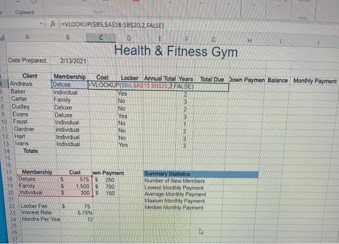
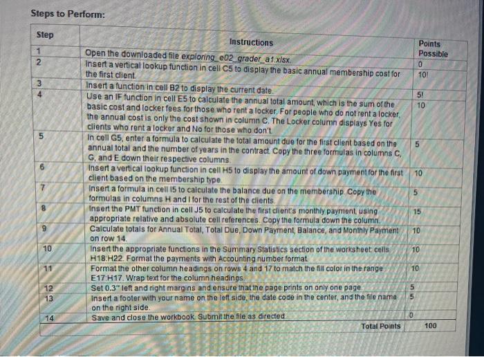
Clipboard Son Ideas fx =VLOOKUP(SB5,SA$18:$B$20,2,FALSE) B D H Health & Fitness Gym Date Prepared 2/13/2021 No NO Client Membership Cost Locker Annual Total Years Total Due Down Paymen Balance Monthly Payment 5 Andrews Deluxe FVLOOKUP(585, SAS18 SB320 2 FALSE) 6 Baker Individual Yes 2 7 Carter Family 8 Dudley Deluxe No 2 9 Evans Deluxe Yes 10 Foust Individual 11 Gardner Individual No 12 Hart Individual No 13 Ivans Individual Yes Totals 15 16 12 Membership Cost wn Payment Summary Statistics 18 Deluxe $ 575$ 250 Number of New Members 19 Family 1,500S 700 Lowest Monthly Payment 20 individual $ 300 $ 150 Average Monthly Payment 21 Maxum Monthly Payment 22 Locker Fee 75 Median Monthly Payment interest Rate 575% 24 Months Per Year 12 AAA $ Steps to Perform: Step 1 2 Points Possible 0 101 3 4 5! 10 5 5 10 Instructions Open the downloaded file exploring_e02_grader_a1.xlsx Insert a vertical lookup function in cell C5 to display the basic annual membership cost for the first client Insert a function in cell B2 to display the current date. Use an IF function in cell ES to calculate the annual total amount, which is the sum of the basic cost and locker fees for those who rent a locker. For people who do not rent a locker, the annual cost is only the cost shown in column C. The Locker column displays Yes for clients who rent a locker and No for those who don't In cell G5, enter a formula to calculate the total amount due for the first client based on the annual total and the number of years in the contract Copy the three formulas in columns C. G, and E down their respective columns Insert a vertical lookup function in cell H5 to display the amount of down payment for the first client based on the membership type. Insert a formula in cell 15 to calculate the balance due on the membership Copy the formulas in columns Hand I for the rest of the clients. Insert the PMT function in cell J5 to calculate the first client's monthly payment using appropriate relative and absolute cell references. Copy the formula down the column Calculate totals for Annual Total, Total Due, Down Payment , Balance, and Monthly Payment on row 14 Insert the appropriate functions in the Summary Statistics section of the worksheet cells H18.H22. Format the payments with Accounting number format Format the other column headings on rows 4 and 17 to match the fill color in the range E17:H17 Wrap text for the column headings Set 0.3" left and right margins and ensure that ine page prints on only one page Insert a footer with your name on the left side, the date code in the center, and the file name on the right side. Save and close the workbook Submit the file as directed Total Points 7 5 8 15 9 10 10 10 11 10 12 13 5 5 14 0 100