HELP PLEASE

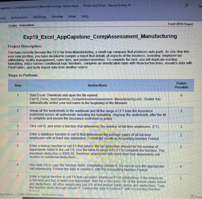
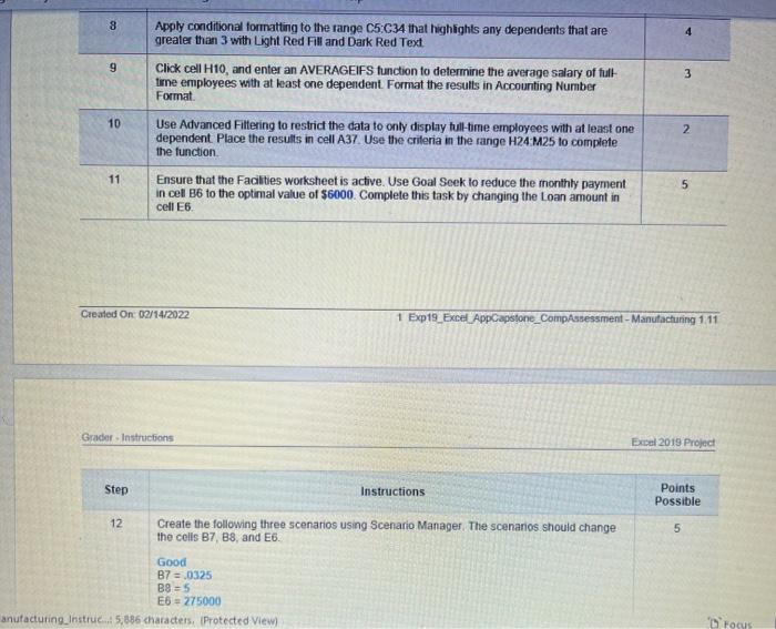
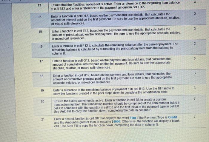
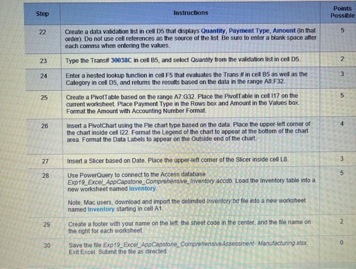
o Jus Capstone CompAssessment Manufacturing Instructions - Protected ViewSaved to this PC References out Mailings Review View Help Grader-Instructions Excel 2019 Project Exp19_Excel_AppCapstone_CompAssessment_Manufacturing Project Description: You have recently become the CFO for Beta Manufacturing, a small cap company that produces auto parts. As you step into your new position, you have decided to compile a report that details all aspects of the business, including employee tax withholding, facility management, sales data, and product inventory. To complete the task, you will duplicate existing formatting, utilize various conditional logic functions, complete an arnortization table with financial functions, visualize data with PivotTables, and lastly import data from another source Steps to Perform: Step Instructions Points Possible 0 2 3 3 3 4 2 1 Start Excel Download and open the file named Exp19_Excel AppCapstone_ComprehensiveAssessment- Manufacturing xlsx Grader has automatically added your last name to the beginning of the filename. Group all the worksheets in the workbook and fill the range A1 F1 from the Insurance worksheet across all worksheets including the formatting. Ungroup the worksheets after the fill is complete and ensure the Insurance worksheet is active. 3 Click cell 15, and enter a function that determines the number of full-time employees, (FT). Enter a database function in cell 16 that determines the average salary of all full-time employees with at least one dependent Format the results in Accounting Number Format Enter a lookup function in cell Es that returns the tax deduction amount for the number of dependents listed in the cell C5 Use the table in range H13:117 to complete the function. The maximum deduction is $500.00, therefore, employees with more than four dependents will receive no additional deductions 6 Use Auto Fill to copy the function down, completing column E. Be sure to use the appropriate cell referencing. Format the data in column with the Accounting Number Format Enter a logical function in cell F5 that calculates employee FICA withholding If the employee is full-time and has at least one dependent, then he or she pays 7% of the annual salary minus any deductions. All other employees pay 5% of the annual salary minus any deductions Copy the function down through column F Format the data in column F with Accounting Number mg_lostru...15,886 characters. (Protected View 5 2 7 3 Carm D FOCU 8 9 3 Apply conditional formatting to the range C5:C34 that highlights any dependents that are greater than 3 with Light Red Fill and Dark Red Text Click cell H10, and enter an AVERAGEIFS function to determine the average salary of full time employees with at least one dependent Format the results in Accounting Number Format. Use Advanced Filtering to restrict the data to only display tull-time employees with at least one dependent Place the results in cell A37. Use the criteria in the range H24 M25 to complete the function Ensure that the Facilities worksheet is active. Use Goal Seek to reduce the monthly payment in cel 86 to the optimal value of $6000. Complete this task by changing the Loan amount in cell E6 10 2 11 5 Created On: 02/14/2022 1 Exp19 Excel AppCapstone_CompAssessment - Manufacturing 111 Grader. Instructions Excel 2019 Project Step Instructions Points Possible 12 5 Create the following three scenarios using Scenario Manager. The scenarios should change the cells B7, B8, and E6. Good B7 = .0325 B9 = 5 E5 = 275000 anufacturing Instruc... 5,886 characters. Protected View) 'D Focus 13 3 14 3 15 2 16 3 17 Ensure that the Facilities worksheet is active Enter a reference to the beginning loan balance in cel B12 and enter a reference to the payment amount in cel C12. Enter a function in cell D12, based on the payment and loan details, that calculates the amount of interest paid on the first payment. Be sure to use the appropriate absolute, relative, or mixed cell references Enter a function in cell E12, based on the payment and loan details, that calculates the amount of principal paid on the first payment. Be sure to use the appropriate absolute, relative, of mixed cell references Enter a formula in cell F 12 to calculate the remaining balance after the current payment. The remaining balance is calculated by subtracting the principal payment from the balance in column B. Enter a function in cell G12, based on the payment and loan details, that calculates the amount of cumulative interest paid on the first payment. Be sure to use the appropriate absolute, relative, or mixed cell references. Enter a function in cell H12, based on the payment and loan details, that calculates the amount of cumulative principal paid on the first payment. Be sure to use the appropriate absolute, relative, or mixed cell references. Enter a reference to the remaining balance of payment 1 in cell B13. Use the fill handle to copy the functions created in the prior steps down to complete the amortization table. Ensure the Sales worksheet is active Enter a function in cell B8 to create a custom transaction number. The transaction number should be comprised of the item number listed in cell C combined with the quantity in cell D8 and the first initial of the payment type in cell E8. Use Auto Fill to copy the function down, completing the data in column B Enter a nested function in cell G8 that displays the word Flag of the Payment Type is Credit and the Amount is greater than or equal to $4000. Otherwise, the function will display a blank cell Use Auto Fill to copy the function down, completing the data in column G 3 18 3 19 7 20 7 21 Step Instructions Points Possible 22 5 23 2 24 3 Create a data validation list in cell D5 that displays Quantity, Payment Type, Amount (in that order). Do not use cell references as the source of the list Be sure to enter a blank space after each comma when entering the values. Type the Trans# 30038C in cell B5, and select Quantity from the validation list in cell 05. Enter a nested lookup function in cell F5 that evaluates the Trans #in cell B5 as well as the Categbry in cell D5, and returns the results based on the data in the range A8: F32. Create a PivotTable based on the range AT:G32. Place the PivotTable in cell 117 on the current worksheet. Place Payment Type in the Rows box and Amount in the Values box Format the Amount with Accounting Number Format. Insert a PivotChart using the Pie chart type based on the data. Place the upper-left corner of the chart inside cell 122. Format the Legend of the chart to appear at the bottom of the chart area. Format the Data Labels to appear on the outside end of the chart. 5 25 4 4 26 27 3 5 28 Insert a Slicer based on Date Place the upper-left corner of the Slicer inside cell L8. Use PowerQuery to connect to the Access database Exp19_Excel_App Capstone_Comprehensive_Inventory accdb. Load the inventory table into a new worksheet named Inventory. Note, Mac users, download and import the delimited Inventory.txt file into a new worksheet named Inventory starting in cell A1. Create a footer with your name on the left, the sheet code in the center, and the file name on the right for each worksheet. Save the file Exp19_Excel_App Capstone_Comprehensive Assessment- Manufacturing.xlsx Exit Excel Submit the file as directed 2 29 0 30 o Jus Capstone CompAssessment Manufacturing Instructions - Protected ViewSaved to this PC References out Mailings Review View Help Grader-Instructions Excel 2019 Project Exp19_Excel_AppCapstone_CompAssessment_Manufacturing Project Description: You have recently become the CFO for Beta Manufacturing, a small cap company that produces auto parts. As you step into your new position, you have decided to compile a report that details all aspects of the business, including employee tax withholding, facility management, sales data, and product inventory. To complete the task, you will duplicate existing formatting, utilize various conditional logic functions, complete an arnortization table with financial functions, visualize data with PivotTables, and lastly import data from another source Steps to Perform: Step Instructions Points Possible 0 2 3 3 3 4 2 1 Start Excel Download and open the file named Exp19_Excel AppCapstone_ComprehensiveAssessment- Manufacturing xlsx Grader has automatically added your last name to the beginning of the filename. Group all the worksheets in the workbook and fill the range A1 F1 from the Insurance worksheet across all worksheets including the formatting. Ungroup the worksheets after the fill is complete and ensure the Insurance worksheet is active. 3 Click cell 15, and enter a function that determines the number of full-time employees, (FT). Enter a database function in cell 16 that determines the average salary of all full-time employees with at least one dependent Format the results in Accounting Number Format Enter a lookup function in cell Es that returns the tax deduction amount for the number of dependents listed in the cell C5 Use the table in range H13:117 to complete the function. The maximum deduction is $500.00, therefore, employees with more than four dependents will receive no additional deductions 6 Use Auto Fill to copy the function down, completing column E. Be sure to use the appropriate cell referencing. Format the data in column with the Accounting Number Format Enter a logical function in cell F5 that calculates employee FICA withholding If the employee is full-time and has at least one dependent, then he or she pays 7% of the annual salary minus any deductions. All other employees pay 5% of the annual salary minus any deductions Copy the function down through column F Format the data in column F with Accounting Number mg_lostru...15,886 characters. (Protected View 5 2 7 3 Carm D FOCU 8 9 3 Apply conditional formatting to the range C5:C34 that highlights any dependents that are greater than 3 with Light Red Fill and Dark Red Text Click cell H10, and enter an AVERAGEIFS function to determine the average salary of full time employees with at least one dependent Format the results in Accounting Number Format. Use Advanced Filtering to restrict the data to only display tull-time employees with at least one dependent Place the results in cell A37. Use the criteria in the range H24 M25 to complete the function Ensure that the Facilities worksheet is active. Use Goal Seek to reduce the monthly payment in cel 86 to the optimal value of $6000. Complete this task by changing the Loan amount in cell E6 10 2 11 5 Created On: 02/14/2022 1 Exp19 Excel AppCapstone_CompAssessment - Manufacturing 111 Grader. Instructions Excel 2019 Project Step Instructions Points Possible 12 5 Create the following three scenarios using Scenario Manager. The scenarios should change the cells B7, B8, and E6. Good B7 = .0325 B9 = 5 E5 = 275000 anufacturing Instruc... 5,886 characters. Protected View) 'D Focus 13 3 14 3 15 2 16 3 17 Ensure that the Facilities worksheet is active Enter a reference to the beginning loan balance in cel B12 and enter a reference to the payment amount in cel C12. Enter a function in cell D12, based on the payment and loan details, that calculates the amount of interest paid on the first payment. Be sure to use the appropriate absolute, relative, or mixed cell references Enter a function in cell E12, based on the payment and loan details, that calculates the amount of principal paid on the first payment. Be sure to use the appropriate absolute, relative, of mixed cell references Enter a formula in cell F 12 to calculate the remaining balance after the current payment. The remaining balance is calculated by subtracting the principal payment from the balance in column B. Enter a function in cell G12, based on the payment and loan details, that calculates the amount of cumulative interest paid on the first payment. Be sure to use the appropriate absolute, relative, or mixed cell references. Enter a function in cell H12, based on the payment and loan details, that calculates the amount of cumulative principal paid on the first payment. Be sure to use the appropriate absolute, relative, or mixed cell references. Enter a reference to the remaining balance of payment 1 in cell B13. Use the fill handle to copy the functions created in the prior steps down to complete the amortization table. Ensure the Sales worksheet is active Enter a function in cell B8 to create a custom transaction number. The transaction number should be comprised of the item number listed in cell C combined with the quantity in cell D8 and the first initial of the payment type in cell E8. Use Auto Fill to copy the function down, completing the data in column B Enter a nested function in cell G8 that displays the word Flag of the Payment Type is Credit and the Amount is greater than or equal to $4000. Otherwise, the function will display a blank cell Use Auto Fill to copy the function down, completing the data in column G 3 18 3 19 7 20 7 21 Step Instructions Points Possible 22 5 23 2 24 3 Create a data validation list in cell D5 that displays Quantity, Payment Type, Amount (in that order). Do not use cell references as the source of the list Be sure to enter a blank space after each comma when entering the values. Type the Trans# 30038C in cell B5, and select Quantity from the validation list in cell 05. Enter a nested lookup function in cell F5 that evaluates the Trans #in cell B5 as well as the Categbry in cell D5, and returns the results based on the data in the range A8: F32. Create a PivotTable based on the range AT:G32. Place the PivotTable in cell 117 on the current worksheet. Place Payment Type in the Rows box and Amount in the Values box Format the Amount with Accounting Number Format. Insert a PivotChart using the Pie chart type based on the data. Place the upper-left corner of the chart inside cell 122. Format the Legend of the chart to appear at the bottom of the chart area. Format the Data Labels to appear on the outside end of the chart. 5 25 4 4 26 27 3 5 28 Insert a Slicer based on Date Place the upper-left corner of the Slicer inside cell L8. Use PowerQuery to connect to the Access database Exp19_Excel_App Capstone_Comprehensive_Inventory accdb. Load the inventory table into a new worksheet named Inventory. Note, Mac users, download and import the delimited Inventory.txt file into a new worksheet named Inventory starting in cell A1. Create a footer with your name on the left, the sheet code in the center, and the file name on the right for each worksheet. Save the file Exp19_Excel_App Capstone_Comprehensive Assessment- Manufacturing.xlsx Exit Excel Submit the file as directed 2 29 0 30