help to on the questions for Excel

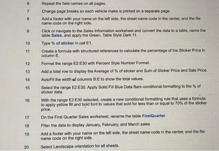
6 Repeat the field names on all pages. 7 Change page breaks so each vehicle make is printed on a separate page. 8 Add a footer with your name on the left side, the sheet name code in the center, and the file name code on the right side. 9 Click or navigate to the Sales Information worksheet and convert the data to a table, name the table Sales, and apply the Green, Table Style Dark 11. 10 Type \% of sticker in cell E1. 11 Create a formula with structured references to calculate the percentage of the Sticker Price in column E. 12 Format the range E2:E30 with Percent Style Number Format. 13 Add a total row to display the Average of \% of sticker and Sum of Sticker Price and Sale Price. 14 AutoFit the width of columns B : E to show the total values. 15 Select the range E2:E30. Apply Solid Fill Blue Data Bars conditional formatting to the \% of sticker data. 16 With the range E2:E30 selected, create a new conditional formatting rule that uses a formula to apply yellow fill and bold font to values that sold for less than or equal to 70% of the sticker price. 17 On the First Quarter Sales worksheet, rename the table FirstQuarter. 18 Filter the data to display January, February, and March sales. 19 Add a footer with your name on the left side, the sheet name code in the center, and the file name code on the right side. 20 Select Landscape orientation for all sheets. 6 Repeat the field names on all pages. 7 Change page breaks so each vehicle make is printed on a separate page. 8 Add a footer with your name on the left side, the sheet name code in the center, and the file name code on the right side. 9 Click or navigate to the Sales Information worksheet and convert the data to a table, name the table Sales, and apply the Green, Table Style Dark 11. 10 Type \% of sticker in cell E1. 11 Create a formula with structured references to calculate the percentage of the Sticker Price in column E. 12 Format the range E2:E30 with Percent Style Number Format. 13 Add a total row to display the Average of \% of sticker and Sum of Sticker Price and Sale Price. 14 AutoFit the width of columns B : E to show the total values. 15 Select the range E2:E30. Apply Solid Fill Blue Data Bars conditional formatting to the \% of sticker data. 16 With the range E2:E30 selected, create a new conditional formatting rule that uses a formula to apply yellow fill and bold font to values that sold for less than or equal to 70% of the sticker price. 17 On the First Quarter Sales worksheet, rename the table FirstQuarter. 18 Filter the data to display January, February, and March sales. 19 Add a footer with your name on the left side, the sheet name code in the center, and the file name code on the right side. 20 Select Landscape orientation for all sheets