Here is the excel sheet I am working on. Could you please explain to me how to do part F&G with the data in my excel spreadsheet posted below.

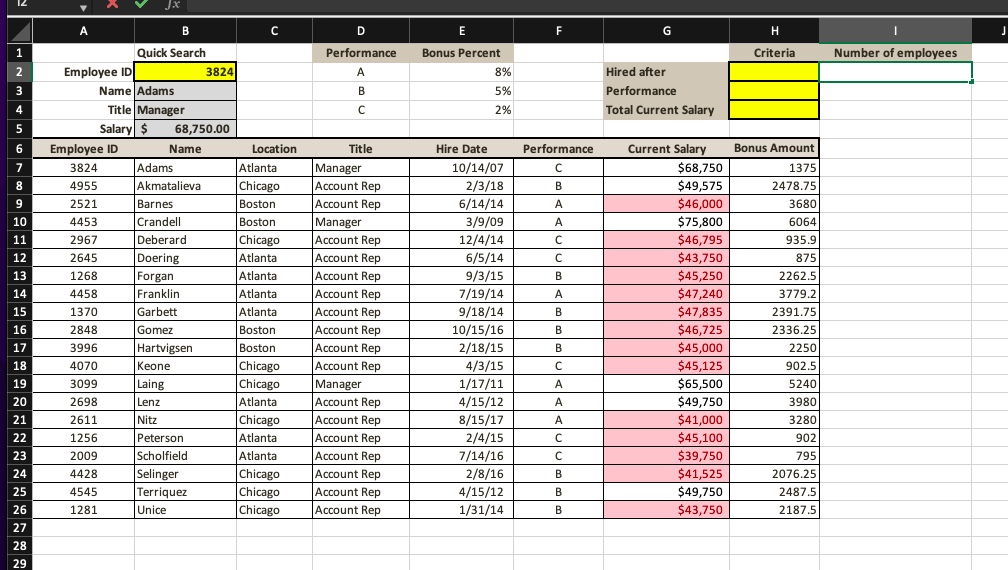
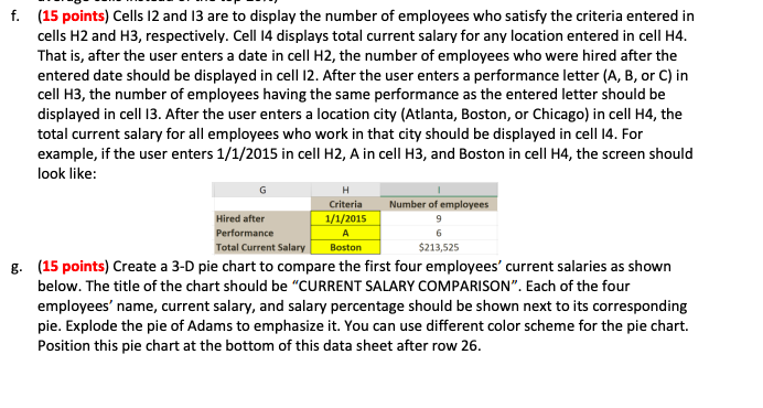
f. (15 points) Cells 12 and 13 are to display the number of employees who satisfy the criteria entered in cells H2 and H3, respectively. Cell 14 displays total current salary for any location entered in cell H4. That is, after the user enters a date in cell H2, the number of employees who were hired after the entered date should be displayed in cell I2. After the user enters a performance letter (A, B, or C) in cell H3, the number of employees having the same performance as the entered letter should be displayed in cell I3. After the user enters a location city (Atlanta, Boston, or Chicago) in cell H, the total current salary for all employees who work in that city should be displayed in cell 14 . For example, if the user enters 1/1/2015 in cell H2,A in cell H3, and Boston in cell H4, the screen should look like: g. (15 points) Create a 3-D pie chart to compare the first four employees' current salaries as shown below. The title of the chart should be "CURRENT SALARY COMPARISON". Each of the four employees' name, current salary, and salary percentage should be shown next to its corresponding pie. Explode the pie of Adams to emphasize it. You can use different color scheme for the pie chart. Position this pie chart at the bottom of this data sheet after row 26