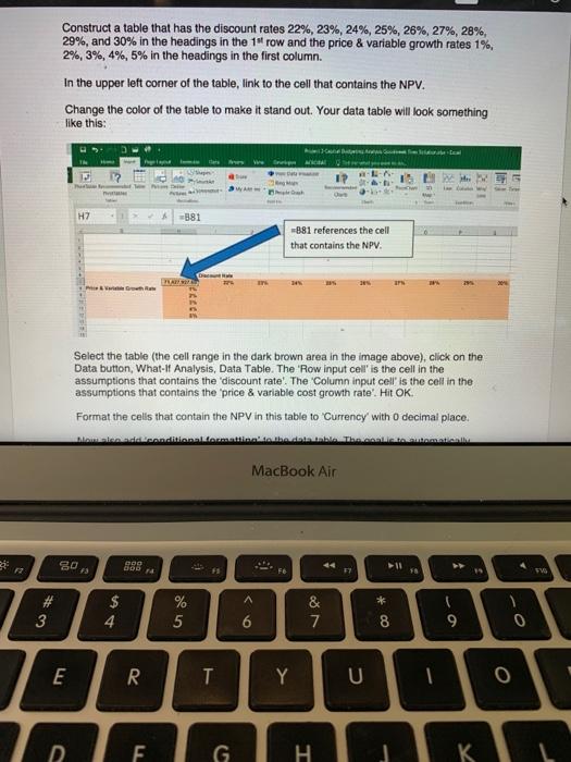
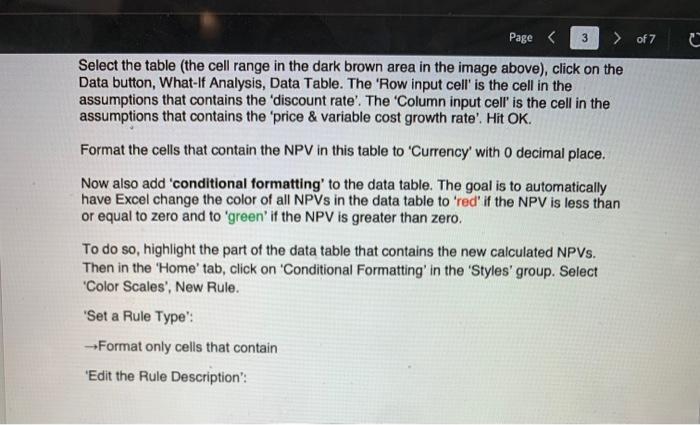
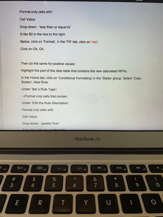
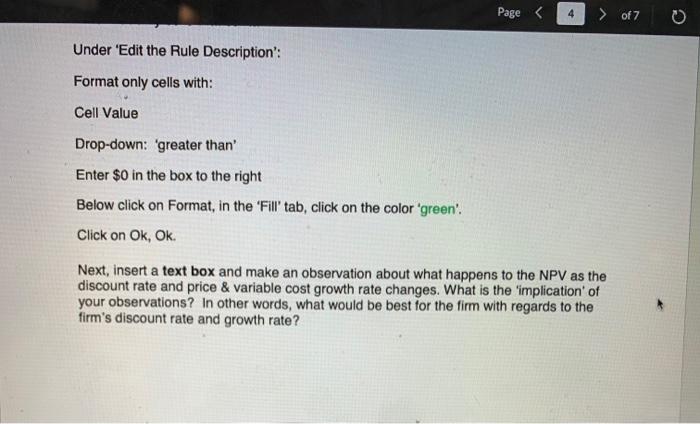
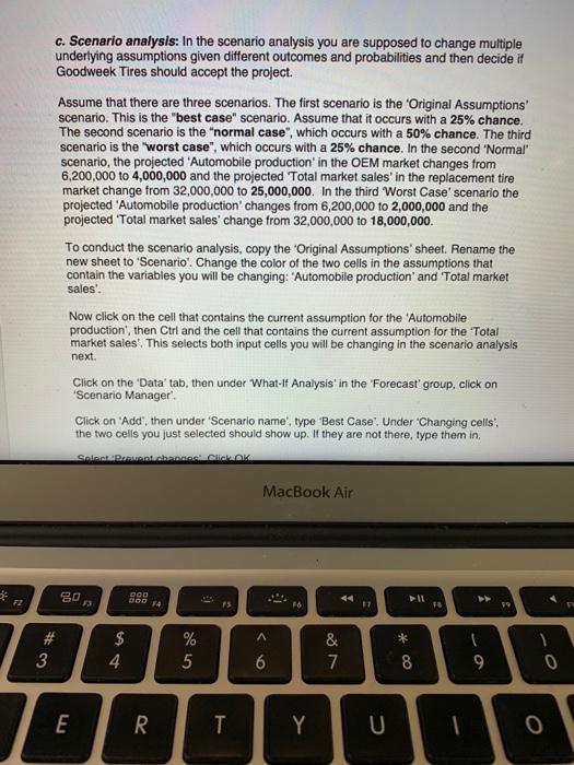
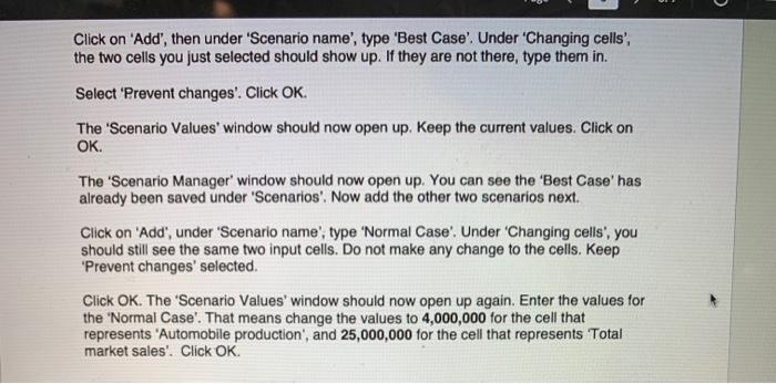
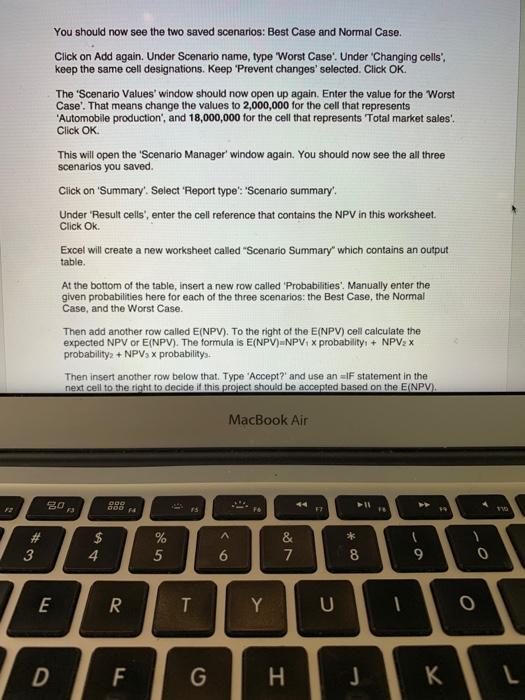
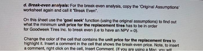
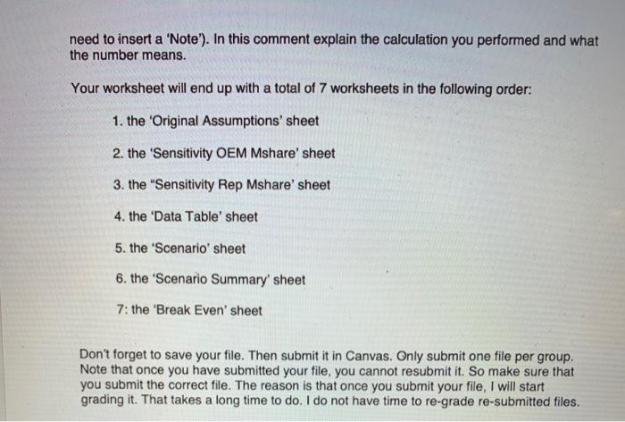
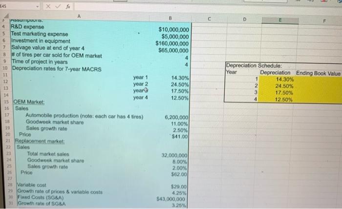
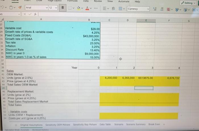
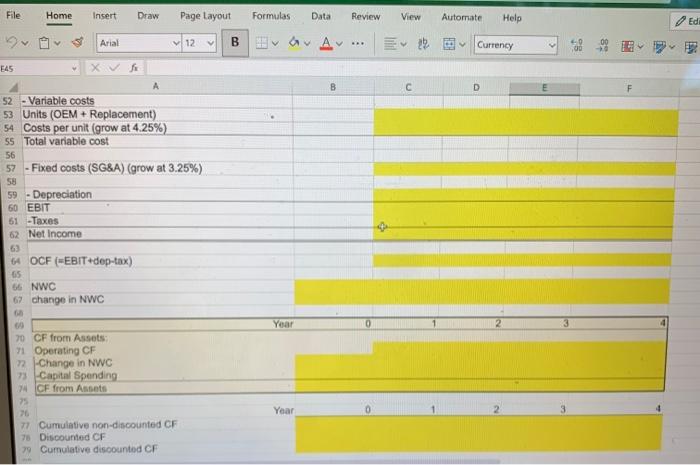
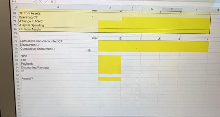
Page 1 > o 1. Original Assumptions: Please read through the Goodweek Tires, Inc. case study at the end of Ch. 6 in your text book (p. 204). The assumptions are all summarized in the Excel workbook template that is attached to this assignment in the 'Original Assumptions' worksheet. Use the first worksheet to calculate the net present value (NPV), internal rate of return (IRR), payback, discounted payback, and profitability index (PI). Make sure your model is 'dynamic'. Then decide if Goodweek Tires should accept the project based on the NPV (using the =IF function). Note: All your answers will be written into this Excel workbook. 2. Risk Analysis: Next you will perform a sensitivity, scenario and break-even analysis and use the data table tool. You will create copies of the 'Original Assumptions' worksheet to perform each of the following analysis: a. Sensitivity analysis: In the sensitivity analysis you are supposed to find out if the NPV is more sensitive to the OEM tire market share or the replacement tire market share. To do that, first copy the Original Assumptions sheet and rename the copied sheet 'Sensitivity OEM Mshare'. On this new sheet, change the OEM tire market share from 11.00% to 12.10% (a 10% increase). Change the color of the cell you changed and add a comment to this cell to explain what you did. Calculate how sensitive the NPV measure is to this 10% increase in the OEM tire market share. Remember that you first have to calculate the % change in the NPV and the % change in the market share. The formula for the % change is =(ending value- beginning value)/beginning value. Then divide the two % changes by each other to find the sensitivity. Note: be careful to format the sensitivity correctly. It should be formatted as a number (not a percent). Use 2 decimals for the sensitivity. Please enter all your sensitivity calculations on the top right area of this sheet. Then add a text box. Note: To insert a text box, go to the 'Insert' button, 'Illustrations" group, under 'Shapes', 'Basic Shapes', select Text Box'. Draw the text box and start typing in it. You can later expand it to fit and show all the text. Change the color of the textbook to make it stand out. In this text box explain in specific terms what the interpretation of this sensitivity is. (For each 1% change in... the...changes by...%) Next, copy the 'Original Assumptions', sheet again. Rename this sheet to 'Sensitivity Rep Mshare'. On this new sheet, change the replacement tire market share from 8.00% to 8.80% (a 10% increase). Again, change the color of the cell you changed and add a comment to this cell to explain what you did. Calculate how sensitive the NPV measure is to this 10% increase in the replacement tire market share. Please enter all your calculations on the top right area of this sheet and highlight them in a different color so that they are easily visible. Add a text box and explain in specific terms what the interpretation of this sensitivity is. 80 F2 13 #3 3 54 4 000 600 14 % 25 MacBook Air F6 44 +11 F7 FA 9 > & 6 28 * 7 8 9 E R T Y U 0 F10 Add a text box and explain in specific terms what the interpretation of this sensitivity is. Compare the two sensitivities and describe what the implications of your findings from the two sensitivity analysis are. Please write your answer in a text box on the 'Sensitivity Rep Mshare' worksheet underneath the sensitivity calculation. b. Data Table: Next, perform an analysis with a two-dimensional 'Data Table'. For this analysis, copy the 'Original Assumptions' sheet again. Rename it to 'Data Table'. You will use the 'Data Table' function to calculate the NPVS for different 'price & variable growth rates' and different 'discount rates'. Construct a table that has the discount rates 22%, 23%, 24%, 25%, 26%, 27%, 28%, 29%, and 30% in the headings in the 1st row and the price & variable growth rates 1%, 2%, 3%, 4%, 5% in the headings in the first column. In the upper left corner of the table, link to the cell that contains the NPV. Change the color of the table to make it stand out. Your data table will look something like this: H7 =881 881 references the cell that contains the NPV. #3 Select the table (the cell range in the dark brown area in the image above), click on the Data button, What-If Analysis, Data Table. The 'Row input cell' is the cell in the assumptions that contains the 'discount rate'. The 'Column input cell' is the cell in the assumptions that contains the 'price & variable cost growth rate. Hit OK. Format the cells that contain the NPV in this table to 'Currency' with 0 decimal place. Now also add conditional formatting to the data aticall 80 43 000 800 14 MacBook Air 44 11 54 85 % & 6 27 * 8 9 0 E R T Y U 0 G H K FIG Page < 3 > of 7 Select the table (the cell range in the dark brown area in the image above), click on the Data button, What-If Analysis, Data Table. The 'Row input cell' is the cell in the assumptions that contains the 'discount rate'. The 'Column input cell' is the cell in the assumptions that contains the 'price & variable cost growth rate'. Hit OK. Format the cells that contain the NPV in this table to 'Currency' with 0 decimal place. Now also add 'conditional formatting' to the data table. The goal is to automatically have Excel change the color of all NPVS in the data table to 'red' if the NPV is less than or equal to zero and to 'green' if the NPV is greater than zero. To do so, highlight the part of the data table that contains the new calculated NPVs. Then in the 'Home' tab, click on 'Conditional Formatting' in the 'Styles' group. Select 'Color Scales', New Rule. 'Set a Rule Type': Format only cells that contain 'Edit the Rule Description": C Format only cells with: Cell Value Drop-down: 'less than or equal to' Enter $0 in the box to the right Below, click on 'Format', in the 'Fill' tab, click on 'red'. Click on Ok, Ok. Then do the same for positive values: Highlight the part of the data table that contains the new calculated NPVS. In the Home tab, click on 'Conditional Formatting' in the 'Styles' group. Select 'Color Scales', New Rule. Under 'Set a Rule Type': Format only cells that contain Under 'Edit the Rule Description": Format only cells with: Cell Value Drop-down: 'greater than FZ 80 9 $ 54 #3 3 EL E 000 800 74 R MacBook Air 44 F7 114 4 25 % 6 27 & * 7 8 9 T Y 0 Page < > of 7 Under 'Edit the Rule Description': Format only cells with: Cell Value Drop-down: 'greater than' Enter $0 in the box to the right Below click on Format, in the 'Fill' tab, click on the color 'green'. Click on Ok, Ok. Next, insert a text box and make an observation about what happens to the NPV as the discount rate and price & variable cost growth rate changes. What is the 'implication' of your observations? In other words, what would be best for the firm with regards to the firm's discount rate and growth rate? C 72 c. Scenario analysis: In the scenario analysis you are supposed to change multiple underlying assumptions given different outcomes and probabilities and then decide if Goodweek Tires should accept the project. Assume that there are three scenarios. The first scenario is the 'Original Assumptions' scenario. This is the "best case" scenario. Assume that it occurs with a 25% chance. The second scenario is the "normal case", which occurs with a 50% chance. The third scenario is the "worst case", which occurs with a 25% chance. In the second "Normal" scenario, the projected 'Automobile production' in the OEM market changes from 6,200,000 to 4,000,000 and the projected Total market sales' in the replacement tire market change from 32,000,000 to 25,000,000. In the third 'Worst Case' scenario the projected 'Automobile production' changes from 6,200,000 to 2,000,000 and the projected 'Total market sales' change from 32,000,000 to 18,000,000. To conduct the scenario analysis, copy the 'Original Assumptions' sheet. Rename the new sheet to 'Scenario'. Change the color of the two cells in the assumptions that contain the variables you will be changing: "Automobile production' and 'Total market sales'. Now click on the cell that contains the current assumption for the "Automobile production, then Ctrl and the cell that contains the current assumption for the Total market sales'. This selects both input cells you will be changing in the scenario analysis next. Click on the 'Data' tab, then under "What-If Analysis' in the 'Forecast' group, click on 'Scenario Manager. Click on 'Add', then under 'Scenario name', type 'Best Case'. Under 'Changing cells', the two cells you just selected should show up. If they are not there, type them in. Select Prevent changes Click OK MacBook Air 80 13 # #3 3 $ 54 4 LL E 000 600 F4 F6 44 17 6 & 7 * 7 8 9 % 25 ^ R T Y U 0 Click on 'Add', then under 'Scenario name', type 'Best Case'. Under 'Changing cells', the two cells you just selected should show up. If they are not there, type them in. Select 'Prevent changes'. Click OK. The 'Scenario Values' window should now open up. Keep the current values. Click on OK. The 'Scenario Manager' window should now open up. You can see the 'Best Case' has already been saved under 'Scenarios'. Now add the other two scenarios next. Click on 'Add', under 'Scenario name', type 'Normal Case'. Under 'Changing cells', you should still see the same two input cells. Do not make any change to the cells. Keep 'Prevent changes' selected. Click OK. The 'Scenario Values' window should now open up again. Enter the values for the 'Normal Case'. That means change the values to 4,000,000 for the cell that represents 'Automobile production', and 25,000,000 for the cell that represents Total market sales'. Click OK. You should now see the two saved scenarios: Best Case and Normal Case. Click on Add again. Under Scenario name, type 'Worst Case'. Under 'Changing cells, keep the same cell designations. Keep 'Prevent changes' selected. Click OK. The 'Scenario Values' window should now open up again. Enter the value for the 'Worst Case'. That means change the values to 2,000,000 for the cell that represents 'Automobile production', and 18,000,000 for the cell that represents Total market sales'. Click OK. This will open the 'Scenario Manager' window again. You should now see the all three scenarios you saved. Click on 'Summary'. Select 'Report type': 'Scenario summary'. Under 'Result cells', enter the cell reference that contains the NPV in this worksheet. Click Ok. Excel will create a new worksheet called "Scenario Summary" which contains an output table. At the bottom of the table, insert a new row called 'Probabilities'. Manually enter the given probabilities here for each of the three scenarios: the Best Case, the Normal Case, and the Worst Case. Then add another row called E(NPV). To the right of the E(NPV) cell calculate the expected NPV or E(NPV). The formula is E(NPV) NPV x probability: + NPV2 x probability + NPV x probabilitys. Then insert another row below that. Type 'Accept?' and use an IF statement in the next cell to the right to decide if this project should be accepted based on the E(NPV). MacBook Air 12 80 000 F3 200 14 $ 54 #3 15 % 95 6 E R T D F G Y H & 87 7 44 FT +11 8 * - 4 9 0 0 K L d. Break-even analysis: For the break-even analysis, copy the 'Original Assumptions' worksheet again and call it "Break Even". On this sheet use the 'goal seek' function (using the original assumptions) to find out what the minimum unit price for the replacement tires has to be in order for Goodweek Tires Inc. to break even (i.e to have an NPV = 0). Change the color of the cell that contains the unit price for the replacement tires to highlight it. Insert a comment in the cell that shows the break-even price. Note, to insert a comment, right click on the cell, Insert Comment. (If you are using a Mac vou will need to insert a 'Note'). In this comment explain the calculation you performed and what the number means. Your worksheet will end up with a total of 7 worksheets in the following order: 1. the 'Original Assumptions' sheet 2. the 'Sensitivity OEM Mshare' sheet 3. the "Sensitivity Rep Mshare' sheet 4. the 'Data Table' sheet 5. the 'Scenario' sheet 6. the 'Scenario Summary' sheet 7: the 'Break Even' sheet Don't forget to save your file. Then submit it in Canvas. Only submit one file per group. Note that once you have submitted your file, you cannot resubmit it. So make sure that you submit the correct file. The reason is that once you submit your file, I will start grading it. That takes a long time to do. I do not have time to re-grade re-submitted files. 645 3 fx B C D Depreciation Schedule: Depreciation Ending Book Value 4 R&D expense 5 Test marketing expense 6 Investment in equipment 7 Salvage value at end of year 4 8 # of tires per car sold for OEM market 9 Time of project in years 10 Depreciation rates for 7-year MACRS $10,000,000 $5,000,000 $160,000,000 $65,000,000 4 4 Year 11 year 1 14.30% 12 year 2 24.50% 13 year 17.50% 14 year 4 12.50% 15 OEM Market: 16 Sales 17 Automobile production (note: each car has 4 tires) 6,200,000 18 Goodweek market share 11.00% 19 Sales growth rate 2.50% 20 Price $41.00 22 Sales 23 21 Replacement market Total market sales 32,000,000 24 Goodweek market share 8.00% 25 Sales growth rate 2.00% 26 Price $62.00 27 28 Variable cost $29.00 29 Growth rate of prices & variable costs 4.25% 30 Fixed Costs (SG&A) $43,000,000 31 Growth rate of SG&A 3.25% 1 14.30% 2 24.50% 3 17.50% 4 12.50% 329 45 27 ben Page Layout Formulas Data Review View Automate Help V Arial 12 B v Av Currency 28 Variable cost $29.00 29 Growth rate of prices & variable costs 4.25% 30 Fixed Costs (SG&A) $43,000,000 31 Growth rate of SG&A 3.25% 23.00% 32 Tax rate 33 Inflation 34 Discount Rate 35 NWC in year 0 36 NWC in years 1-3 as % of sales 37 38 39 3.25% 13.40% $9,000,000 15.00% C D Year 1 2 v 40 Sales 41 OEM Market 42 Units (grow at 2.5%) 43 Price (grows at 4.25%) 44 Total Sales OEM Market 45 46 Replacement Market 47 Units (grow at 2%) 4 Price (grows at 4.25%) 4 Total Sales Replacement Market 50 Total Sales 51 52 Variable costs 53 Units (OEM Replacement) 54 Costs per unit (grow at 4.25%) 6,200,000 6,355,000 6513875.00 6,676,722 Original Assumptions Sensitivity OEM Mahare Sensitivity Rep Mahare Data Table Scenario Scenario Summary Break Even Editing G File Home Insert Draw Page Layout Formulas Data Review View Automate Help Edi Arial 12 B v A Currency E45 A 52 -Variable costs 53 Units (OEM + Replacement) 54 Costs per unit (grow at 4.25%) 55 Total variable cost 56 57 58 59 -Fixed costs (SG&A) (grow at 3.25%) Depreciation 60 EBIT 61 -Taxes 62 Net Income 63 64 OCF (EBIT+dep-tax) 65 66 NWC 67 change in NWC 68 69 70 CF from Assets: 71 Operating CF 72 Change in NWC 73 Capital Spending Year 74 CF from Assets 75 76 Year 77 Cumulative non-discounted CF 78 Discounted CF 79 Cumulative discounted CF B C D E45 8 70 CF from Assets: 71 Operating CF 72 -Change in NWC 73 Capital Spending 74 CF from Assets 75 76 77 Cumulative non-discounted CF 78 Discounted CF 79 Cumulative discounted CF 80 81 NPV 82 IRR 83 Payback 84 Discounted Payback s P 19 Accept? 90 91 92 93 94 05 97 Tudi Year 0