Hi Could someone please proofread my answer to this question and help me write a clear conclusion to the Chi-square test based on results? It is due today and I am having a problem with this, thanks.

QUESTION:

3. Is there any evidence of a relationship between the hospitalization status and air quality?

DATA:

MY ANSWER:

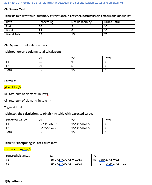
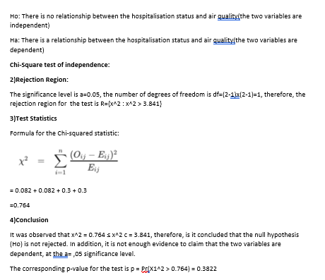
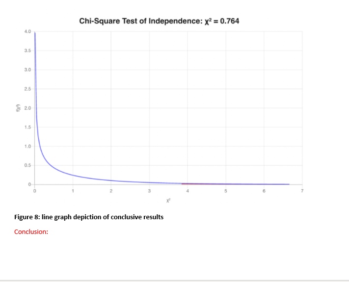
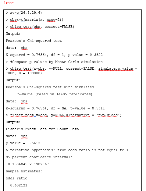
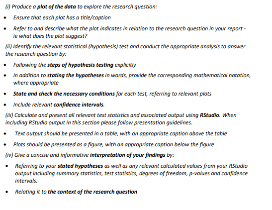
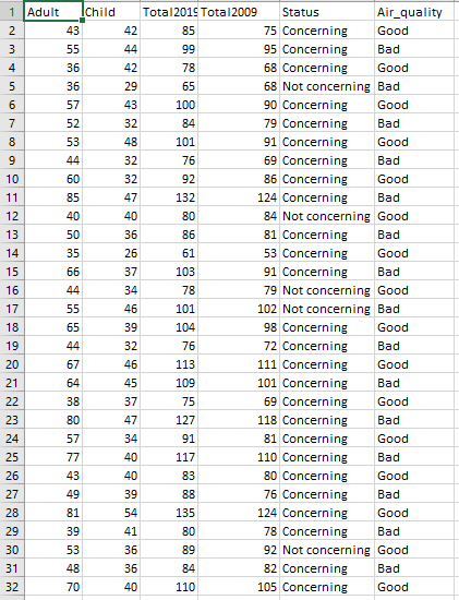
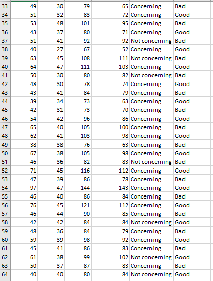
(1) Produce a plot of the data to explore the research question: Ensure that each plot has a title/caption Refer to and describe what the plot indicates in relation to the research question in your report - ie what does the plot suggest? (W) identify the relevant statistical (hypothesis) test and conduct the appropriate analysis to answer the research question by: Following the steps of hypothesis testing explicitly In addition to stating the hypotheses in words, provide the corresponding mathematical notation, where appropriate State and check the necessary conditions for each test, referring to relevant plots Include relevant confidence intervals. (ii) Calculate and present all relevant test statistics and associated output using Studio. When including Studio output in this section please follow presentation guidelines. Text output should be presented in a table, with an appropriate caption above the table Plots should be presented as a figure, with an appropriate caption below the figure (iv) Give a concise and informative interpretation of your findings by: Referring to your stated hypotheses as well as any relevant calculated values from your RStudio output including summary statistics, test statistics, degrees of freedom, p-values and confidence intervals. Relating it to the context of the research question 1 Adult Child Total2019 Total2009 Status Air_quality 2 43 42 85 75 Concerning Good 3 55 44 99 95 Concerning Bad 4 36 42 78 68 Concerning Good 5 36 29 65 68 Not concerning Bad 6 57 43 100 90 Concerning Good 7 52 32 84 79 Concerning Bad 8 53 48 101 91 Concerning Good 9 44 32 76 69 Concerning Bad 10 60 32 92 86 Concerning Good 11 85 47 132 124 Concerning Bad 12 40 40 80 84 Not concerning Good 13 50 36 86 81 Concerning Bad 14 35 26 61 53 Concerning Good 15 66 37 103 91 Concerning Bad 16 44 34 78 79 Not concerning Good 17 55 46 101 102 Not concerning Bad 18 65 39 104 98 Concerning Good 19 44 32 76 72 Concerning Bad 20 67 46 113 111 Concerning Good 21 64 45 109 101 Concerning Bad 22 38 37 75 69 Concerning Good 23 80 47 127 118 Concerning Bad 24 57 34 91 81 Concerning Good 25 77 40 117 110 Concerning Bad 26 43 40 83 80 Concerning Good 27 49 39 88 76 Concerning Bad 28 81 54 135 124 Concerning Good 29 39 41 80 78 Concerning Bad 30 53 36 89 92 Not concerning Good 31 48 36 84 82 Concerning Bad 32 70 40 110 105 Concerning Good 33 34 35 36 37 38 39 40 41 42 43 44 45 46 47 48 49 50 51 52 53 54 55 56 57 58 59 60 61 62 63 64 49 51 53 43 51 40 63 64 50 48 43 39 42 54 65 62 38 67 46 71 47 97 46 76 46 42 30 32 48 37 41 27 45 47 30 30 41 34 31 42 40 41 38 38 36 45 39 47 40 45 44 42 36 39 41 79 83 101 80 92 67 108 111 80 78 84 73 73 96 105 103 76 105 82 116 86 144 86 121 90 84 84 98 86 99 87 80 65 Concerning Bad 72 Concerning Good 95 Concerning Bad 71 Concerning Good 92 Not concerning Bad 52 Concerning Good 111 Not concerning Bad 103 Concerning Good 82 Not concerning Bad 74 Concerning Good 79 Concerning Bad 63 Concerning Good 70 Concerning Bad 86 Concerning Good 100 Concerning Bad 98 Concerning Good 63 Concerning Bad 98 Concerning Good 83 Not concerning Bad 112 Concerning Good 78 Concerning Bad 143 Concerning Good 84 Concerning Bad 112 Concerning Good 85 Concerning Bad 84 Not concerning Good 79 Concerning Bad 92 Concerning Good 83 Concerning Bad 102 Not concerning Good 83 Concerning Bad 84 Not concerning Good 48 59 45 61 50 40 38 37 40 65 66 67 68 69 70 71 62 39 43 47 40 40 35 44 102 74 87 82 79 35 39 40 30 107 Not concerning Bad 73 Concerning Good 83 Concerning Bad 78 Concerning Good 81 Not concerning Bad 80 Concerning Good 72 Not concerning Bad 44 42 84 72 3. Is there any evidence of a relationship between the hospitalisation status and air quality? Chi Square Test: Table 8: Two-way table, summary of relationship between hospitalisation status and air quality Concerning Not Concerning Grand Total Bad 26 9 35 Good 29 6 Grand Total 55 Data 35 70 15 chi-square test of independence: Table 9: Row and column total calculations X1 X2 Total Y1 26 29 55 YZ 9 6 15 Total 35 35 70 Formula: Eli = Ri Ci/T BL: total sum of elements in row ci: total sum of elements in column] T:grand total Table 10: the calculations to obtain the table with expected values Expected Values X1 X2 Total Y1 55 35/70=27.5 55*35/70=27.5 55 YZ 15*35/70=7.5 15*35/70=7.5 15 Total 35 35 70 Table 11: Computing squared distances: Formula: (E-A2/E squared Distances X1 X2 Y1 (26-27.5 42/27.5.0.082 (29-27.5142/27.5 = 0.082 YZ (9-7.5 12/7.5 = 0.3 16 -7.5142/7.5 = 0.3 1) Hypothesis Ho: There is no relationship between the hospitalisation status and air quality/the two variables are independent) Ha: There is a relationship between the hospitalisation status and air quality/the two variables are dependent) Chi-Square test of independence: 2)Rejection Region: The significance level is a=0.05, the number of degrees of freedom is df=(2-11x(2-1)=1, therefore, the rejection region for the test is R={x^2 : x^2>3.841} 3)Test Statistics Formula for the chi-squared statistic: x? , Oj - E.;) Ej Eij = 0.082 +0.082 +0-3+0.3 =0.764 4)Conclusion It was observed that x^2 = 0.764 S x^2 C= 3.841, therefore, is it concluded that the null hypothesis (Ho) is not rejected. In addition, it is not enough evidence to claim that the two variables are dependent, at the a=,05 significance level. The corresponding p-value for the test is p = BOX112 >0.754) = 0.3822 Chi-Square Test of Independence: x2 = 0.764 4.0 3.5 3.0 2.5 8 2.0 1.5 1.0 0.5 Figure 8: line graph depiction of conclusive results Conclusion: R code: WA > X abs chisq.test(obs, correct=FALSE) Output: Pearson's Chi-squared test data: obs X-squared 0.76364, df = 1, p-value = 0.3822 > #Compute p-values by Monte Carlo simulation > chisq.test(x=abe, y=NULL, correct=FALSE, simulate:R:value = TRUE, B = 100000) Output: Pearson's Chi-squared test with simulated p-value (based on le+05 replicates) data: obs X-squared 0.76364, df = NA, p-value = 0.5611 > fisher.test(x=obs, y=NULL, alternative = 'two.sided') Output: Fisher's Exact Test for Count Data data: obs p-value = 0.5613 alternative hypothesis: true odds ratio is not equal to 1 95 percent confidence interval: 0.1536845 2.1982867 sample estimates: odds ratio 0.602121 (1) Produce a plot of the data to explore the research question: Ensure that each plot has a title/caption Refer to and describe what the plot indicates in relation to the research question in your report - ie what does the plot suggest? (W) identify the relevant statistical (hypothesis) test and conduct the appropriate analysis to answer the research question by: Following the steps of hypothesis testing explicitly In addition to stating the hypotheses in words, provide the corresponding mathematical notation, where appropriate State and check the necessary conditions for each test, referring to relevant plots Include relevant confidence intervals. (ii) Calculate and present all relevant test statistics and associated output using Studio. When including Studio output in this section please follow presentation guidelines. Text output should be presented in a table, with an appropriate caption above the table Plots should be presented as a figure, with an appropriate caption below the figure (iv) Give a concise and informative interpretation of your findings by: Referring to your stated hypotheses as well as any relevant calculated values from your RStudio output including summary statistics, test statistics, degrees of freedom, p-values and confidence intervals. Relating it to the context of the research question 1 Adult Child Total2019 Total2009 Status Air_quality 2 43 42 85 75 Concerning Good 3 55 44 99 95 Concerning Bad 4 36 42 78 68 Concerning Good 5 36 29 65 68 Not concerning Bad 6 57 43 100 90 Concerning Good 7 52 32 84 79 Concerning Bad 8 53 48 101 91 Concerning Good 9 44 32 76 69 Concerning Bad 10 60 32 92 86 Concerning Good 11 85 47 132 124 Concerning Bad 12 40 40 80 84 Not concerning Good 13 50 36 86 81 Concerning Bad 14 35 26 61 53 Concerning Good 15 66 37 103 91 Concerning Bad 16 44 34 78 79 Not concerning Good 17 55 46 101 102 Not concerning Bad 18 65 39 104 98 Concerning Good 19 44 32 76 72 Concerning Bad 20 67 46 113 111 Concerning Good 21 64 45 109 101 Concerning Bad 22 38 37 75 69 Concerning Good 23 80 47 127 118 Concerning Bad 24 57 34 91 81 Concerning Good 25 77 40 117 110 Concerning Bad 26 43 40 83 80 Concerning Good 27 49 39 88 76 Concerning Bad 28 81 54 135 124 Concerning Good 29 39 41 80 78 Concerning Bad 30 53 36 89 92 Not concerning Good 31 48 36 84 82 Concerning Bad 32 70 40 110 105 Concerning Good 33 34 35 36 37 38 39 40 41 42 43 44 45 46 47 48 49 50 51 52 53 54 55 56 57 58 59 60 61 62 63 64 49 51 53 43 51 40 63 64 50 48 43 39 42 54 65 62 38 67 46 71 47 97 46 76 46 42 30 32 48 37 41 27 45 47 30 30 41 34 31 42 40 41 38 38 36 45 39 47 40 45 44 42 36 39 41 79 83 101 80 92 67 108 111 80 78 84 73 73 96 105 103 76 105 82 116 86 144 86 121 90 84 84 98 86 99 87 80 65 Concerning Bad 72 Concerning Good 95 Concerning Bad 71 Concerning Good 92 Not concerning Bad 52 Concerning Good 111 Not concerning Bad 103 Concerning Good 82 Not concerning Bad 74 Concerning Good 79 Concerning Bad 63 Concerning Good 70 Concerning Bad 86 Concerning Good 100 Concerning Bad 98 Concerning Good 63 Concerning Bad 98 Concerning Good 83 Not concerning Bad 112 Concerning Good 78 Concerning Bad 143 Concerning Good 84 Concerning Bad 112 Concerning Good 85 Concerning Bad 84 Not concerning Good 79 Concerning Bad 92 Concerning Good 83 Concerning Bad 102 Not concerning Good 83 Concerning Bad 84 Not concerning Good 48 59 45 61 50 40 38 37 40 65 66 67 68 69 70 71 62 39 43 47 40 40 35 44 102 74 87 82 79 35 39 40 30 107 Not concerning Bad 73 Concerning Good 83 Concerning Bad 78 Concerning Good 81 Not concerning Bad 80 Concerning Good 72 Not concerning Bad 44 42 84 72 3. Is there any evidence of a relationship between the hospitalisation status and air quality? Chi Square Test: Table 8: Two-way table, summary of relationship between hospitalisation status and air quality Concerning Not Concerning Grand Total Bad 26 9 35 Good 29 6 Grand Total 55 Data 35 70 15 chi-square test of independence: Table 9: Row and column total calculations X1 X2 Total Y1 26 29 55 YZ 9 6 15 Total 35 35 70 Formula: Eli = Ri Ci/T BL: total sum of elements in row ci: total sum of elements in column] T:grand total Table 10: the calculations to obtain the table with expected values Expected Values X1 X2 Total Y1 55 35/70=27.5 55*35/70=27.5 55 YZ 15*35/70=7.5 15*35/70=7.5 15 Total 35 35 70 Table 11: Computing squared distances: Formula: (E-A2/E squared Distances X1 X2 Y1 (26-27.5 42/27.5.0.082 (29-27.5142/27.5 = 0.082 YZ (9-7.5 12/7.5 = 0.3 16 -7.5142/7.5 = 0.3 1) Hypothesis Ho: There is no relationship between the hospitalisation status and air quality/the two variables are independent) Ha: There is a relationship between the hospitalisation status and air quality/the two variables are dependent) Chi-Square test of independence: 2)Rejection Region: The significance level is a=0.05, the number of degrees of freedom is df=(2-11x(2-1)=1, therefore, the rejection region for the test is R={x^2 : x^2>3.841} 3)Test Statistics Formula for the chi-squared statistic: x? , Oj - E.;) Ej Eij = 0.082 +0.082 +0-3+0.3 =0.764 4)Conclusion It was observed that x^2 = 0.764 S x^2 C= 3.841, therefore, is it concluded that the null hypothesis (Ho) is not rejected. In addition, it is not enough evidence to claim that the two variables are dependent, at the a=,05 significance level. The corresponding p-value for the test is p = BOX112 >0.754) = 0.3822 Chi-Square Test of Independence: x2 = 0.764 4.0 3.5 3.0 2.5 8 2.0 1.5 1.0 0.5 Figure 8: line graph depiction of conclusive results Conclusion: R code: WA > X abs chisq.test(obs, correct=FALSE) Output: Pearson's Chi-squared test data: obs X-squared 0.76364, df = 1, p-value = 0.3822 > #Compute p-values by Monte Carlo simulation > chisq.test(x=abe, y=NULL, correct=FALSE, simulate:R:value = TRUE, B = 100000) Output: Pearson's Chi-squared test with simulated p-value (based on le+05 replicates) data: obs X-squared 0.76364, df = NA, p-value = 0.5611 > fisher.test(x=obs, y=NULL, alternative = 'two.sided') Output: Fisher's Exact Test for Count Data data: obs p-value = 0.5613 alternative hypothesis: true odds ratio is not equal to 1 95 percent confidence interval: 0.1536845 2.1982867 sample estimates: odds ratio 0.602121