Hi, I have a linear Regression Assignment needs help!

I uploaded the assignment and please help me.

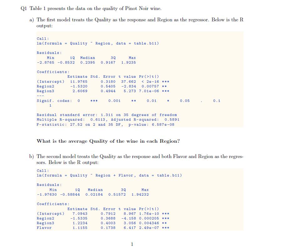
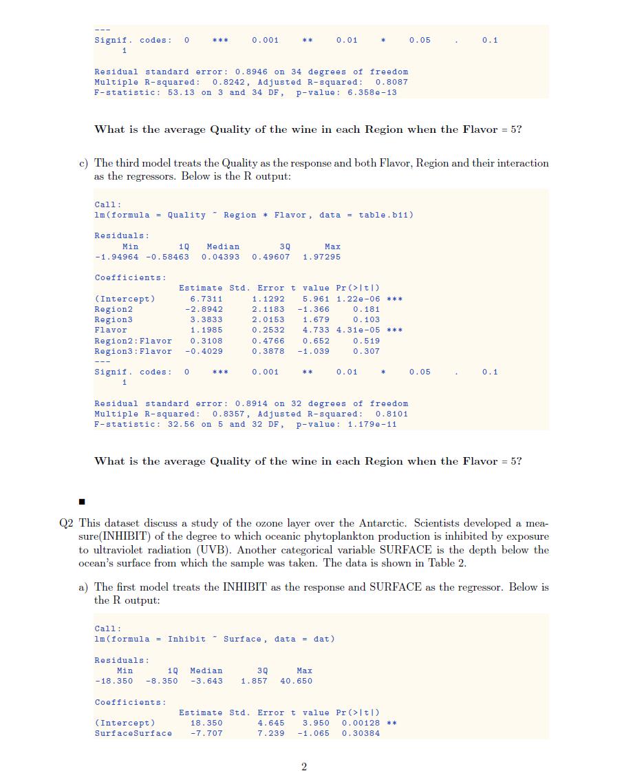
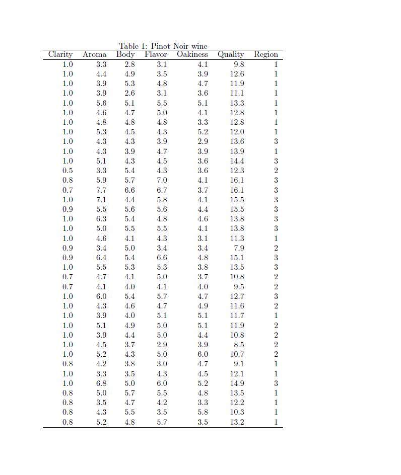
Q1 Table 1 presents the data on the quality of Pinot Noir Wine. a] The rst model treats the Quality as the response and Region as the regressor. Below is the R output: Call: lmtformula = Quality " Region, data = table.b11] Residuals: Min 10 Median 30 Mar 2.8765 0.8532 0.2396 0.916? 1.9235 Coefficients: Estimate Std. Error t value Pr(3|t|) (Intercept) 11.9755 0.3180 37.65: c 2e16 rt: Region2 1.5320 0.5405 2.834 0.00757 it RegionS 2.8069 0.4944 8.273 7.01906 ill Signif. codes: 0 iii 0.001 it 0.01 t 0.05 . 0.1 1 Residual standard error: 1.311 on 55 degrees of freedom Multiple Rsquared: 0.6113JI Ldjusted Rsquared: 0.5391 Fstatistic: 27.52 on 2 and 35 DF, pvalne: 6.537908 What is the average Quality of the wine in each Region? 1):] The second model treats the Quality as the response and both Flavor and Region as the regres sors. Below is the R output: Call: lnformula = Quality " Region + Flavor, data = table.h11} Residuals: Bin 10 Median 30 Mar 1.9?630 0.53844 0.02134 0.61572 1.94232 Coefficients: Estimate Std. Error t value Pr[>|tl) (Intercept) 7.0943 0.7912 8.967 1.75e10 It! RegionZ i.5335 0.3688 4.158 0.000205 it: Regiona 1.2234 0.4003 3.056 0.004346 it Flavor 1.1155 0.1738 6.417 2.49907 III Signif. codes: 0 tit 0.001 it 0.01 t 0.05 . 0.1 1 Residual standard error: 0.3046 on 34 degrees of freedom Hultiple Rsquared: 0.3242, adjusted Rsquared: 0.5057 Fstatistic: 53.13 on 3 and 34 DF, pvalue: 6.353913 What is the average Quality of the wine in each Region when the Flavor = 5? e) The third model treats the Quality as the response and both Flavor. Region and their interaction as the regressors. Belowr is the R output: Call: 1m(ermula = Quality ' Region I Flavor, data = table.bi1} Residuals: Min 10 Hedian 30 Mar 1.94964 0.53463 0.04393 0.49607 1.97295 Coefficients: Estimate Std. Error t value Pr()|tl) (Intercept) 6.7311 1.1292 5.961 1.22906 it: Region2 2.8942 2.1133 1.356 0.131 Regien3 3.3833 2.0153 1.6T9 0.103 Flavor 1.1985 0.2532 4.733 4.31e05 Ill Region2:Flavor 0.3108 0.4756 0.652 0.519 Region3:Flavor 0.4029 0.3878 1.039 0.30? Signif. codes: 0 III 0.001 II 0.01 t 0.05 . 0.1 1 Residual standard error: 0.3914 on 32 degrees of freedom Hultiple Rsquared: 0.835T, deusted squared: 0.3101 Fstatistic: 32.56 on 5 and 32 DF, pvalue: 1.179e11 What is the average Quality of the wine in each Region when the Flavor 2 5? Q2 This dataset discuss a study of the ozone layer over the Antarctic. Scientists developed a mea- sure([N_E|]BIT] of the degree to which oceanic phytoplankton production is inhibited by exposure to ultraviolet radiation (UVB). Another categorical variable SURFACE is the depth below the ocean's surface from which the sample was taken. The data is shown in Table 2. a) The rst model treats the MIBIT as the response and SURFACE as the regressor. Below is the R output: Call: 1m(formn1a = Inhibit ' Surface, data = dat) Residuals: le 10 Median 30 Ear 18.350 3.350 3.643 1.35? 40.650 Coefficients: Estimate Std. Error t value Pr(>|tl) (Intercept) 13.350 4.645 3.950 0.00123 II SurfaceSurface ?.?0T 7.239 1.065 0.30334 Signif. codes: 0 1.0 0.001 it 0.01 t 0.05 . 0.1 1 Residual standard error: 14.69 on 15 degrees of freedom Multiple Rsquared: 0.07026. adjusted Rsquared: 0.008282 Fstatistic: 1.134 on 1 and 15 DF, pvalue: 0.3035 \"That is the average degree of INHIBIT for each SURFACE level? h} The second model treats the INHIBIT as the response and both UVB and SURFACE as the regreesors. Below is the R output: Call: Infornula = Inhibit ' Surface + 085. data = datl Residuals: Min 10 Median 30 Max 13.1210 5.1573 0.65?3 4.2702 25.0790 Coefficients: Estimate Std. Error t value Pr(>|tl) (Intercept) 5.425 4.423 1.22? 0.240151 Snrfacegurface 21.159 5.906 3.533 0.002999 it 095 923.185 218.799 4.219 0.000350 it! Signif. codes: 0 tit 0.001 it 0.01 I 0.05 . 0.1 1 Residual standard error: 10.09 on 14 degrees of freedom Hultiple Rsquared: 0.590T, Adjusted Esquared: 0.5322 Fstatistic: 10.1 on 2 and 14 DF, pvalue: 0.001924 \"mat is the average degree of INHIBIT for each SURFACE level when the UV]?- 2 0.025? c} The third model treats the INHIBIT as the response and both UVB, SURFACE and their interaction as the regressors. Below is the R output: Call: 1ntfornu1a = Inhibit ' Surface I UVB, data = datl Residuals: Min 10 Median 30 Mar 17.9T22 3.9444 0.1806 1.4479 21.0273 Coefficients: Estimate Std. Error t value PrrbltI) (Intercept) 1.181 4.292 0.2T5 0.?8?599 SurfaceSurface 1.2?3 11.056 0.115 0.90983? YB 1226.339 232.7?3 5.269 0.000152 11* SnrfaceSurfece:UVB 939.931 409.339 2.293 0.039134 t Signif. codes: 0 it: 0.001 it 0.01 I 0.05 . 0.1 1 Residual standard error: 3.833 on 13 degrees of freedom Hultiple Rsquared: 0.?086. sdjusted Esquared: 0.5414 Fstatistic: 10.54 on 3 and 13 DF, pvalne: 0.000868 Mat is the average degree of INHIBIT for each SURFACE level when the [TV]?- = 0.025? \fTable 2: czcne hyer Inhibit 0.00 1.00 0.00 100 2.00 2.00 0.00 0.50 10.00 11.00 12.50 14.00 20.00 21.00 25.00 30.00 50.00 U'JE 0.00 0.00 0.01 0.01 0.02 0.03 0.04 0.01 0.00 0.03 0.03 0.01 0.03 0.04 0.02 0.03 003 Surface Deep Deep Deep Surface Surface Surface Surface Deep DEEP Surface Surface Deep Deep Surface Deep Deep Deep