Hi there, Could you help me with this homework? Example 3, 4, and 6 are also attached. Thank you!

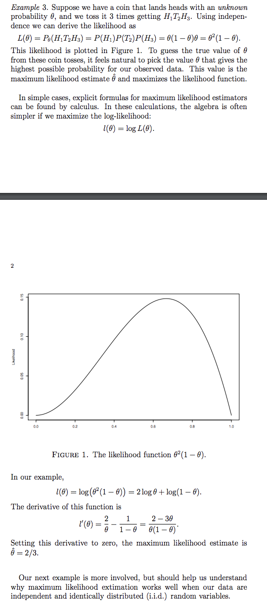
MLE Homework Questions [1) In Example 3 of the notes, consider tossing the coin n times. Assuming the coin is fair, nd the limiting values for l(1;'2)fn and for l(2f3}fn as it gets large. (2) Find I(9) in Example 6 of the notes. Hint: The estimator for HQ} based on observed Fisher information should converge to HQ). Can you nd its limit? (3) Suppose our data are distributed as in Example 4 of the notes, and consider testing 110:9 =1f2 versus 111:3 g 1.32. (a) Derive a formula for the test statistic G'. (b) Suppose we have 50 observations and the sample average is Y = 0.6. What is the value of the test statistic G? (c) With the data in part (b), would you reject the null hy pothesis? What is the approximate pvalue for the test? (4) Suppose our observations 15,. . . ,X\" are i.i.d. with Paw) = FAX =k)= (k+1)92(1_9)k! k: 0:1:2:---: where 9 E [I], 1) is an unknown parameter. (a) Derive an explicit formula for the maximum likelihood es timator 6'. {b} Give a formula for an approximate 95% condence interval for 3. (c) Give the estimate and condence interval from parts (a) and (b) if we have the following 15 observations: 933121013132727. (5) Suppose we have the following 15 observations: 211311212121141, and we model them as i.i.d. variables with distribution 6"\" PM = k) = 'm' k=1,2,..., where 9 E [I], 1) is an unknown parameter. (a) Plot the loglikelihood fmiction in R. (b) Just by looking at the plot, what would you sag,r is the value for the maximum likelihood estimate? Example 3. Suppose we have a coin that lands heads with an unknown probability 9, and we toss it 3 times getting Hngg. Using indepen dence we can derive the likelihood as 15(9) 2 P.9(H1T2H3) = P(H1)P(T2)P(H3) = 9(1 9):; 2 92(1 9). This likelihood is plotted in Figure 1. To gum the true value of 6' from these eoin tomes, it feels natural to pick the value 9 that gives the highest possible probability for our observed data. This value is the maximum likelihood estimate 19 and maximizes the likelihood function. In simple cases, explicit formulas for maximum likelihood estimators can he found by calculus. In these calculations, the algebra is often simpler if we maximize the loglikelihood: as) = 103149). ukuli'loold 0.10 0.15 \".05 (Lil! 00 02 D4 06 08 10 FIGURE 1. The likelihood function 9%] 9). In our example, 1(3) = log [92(1 9}) = Zlog+ log(1 9). The derivative of this function is 2 1 2 39 _ 9 19_ 9(16)' Setting this derivative to zero, the maximum likelihood estimate is 1? = 233. Our next example is more involved, but should help us understand why maximum likelihood extimation works well when our data are independent and identically distributed (i.i.d.} random variables. Example 4. Suppose our observations X1,. . . ,Xn are i.i.d. taking three possible values, I), 1, or 2, with the following probabilities: (lngl #:0; P(X3- = k) 2 23(1 3), k = 1; 92, k = 2. 3 Note that these probabilities have form 9*(1 9)\""' times a constant that depends on lc but is independent of 9. If our observed data are 2:1, . . . , :5\Example 6. Our next example concerns the Poisson distribution, often used to model count data. It will play a central role later in the course in Chapter 7 to study cancer clusters. For this distribution, Po(k) = Po(X = k) = k! k = 0, 1, . .. . Suppose we have i.i.d. observations X1, ...; X, from this distribution. Since log po(k) = log(0*) + log(e-) - log(k!) = klog 0 - 0 - log (k!), 12 we have 1(0) = log Pe( Xk) K=1 = _(Xx log 0 - 0 - log (Xx!)) k=1 = Slog0 - ne - Clog(Xx!), k=1 where, as before, S = Xi+ ... + Xn. Setting I'(0) = - n to zero, the maximum likelihood estimator is 0 =2 = X, n the sample average. Since 1"(0) = S nx A2 observed Fisher information is n F = X' and the approximate 95% confidence interval (7) is (x + 1.96(x) For instance, if we have n = 100 observations and the sample average is X =4, the confidence interval is (4 + 1.96\\/4/100) = (3.608, 4.392)