hopefully these are clear

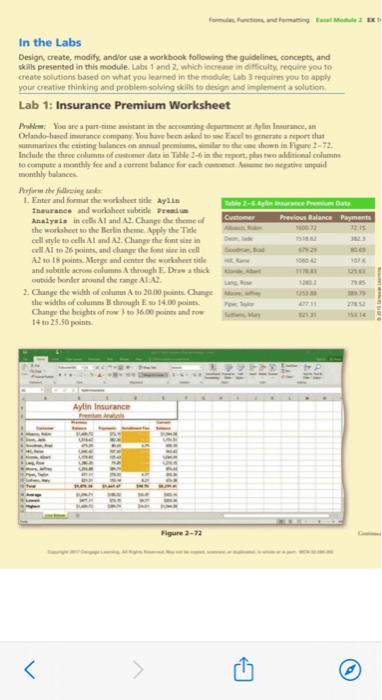
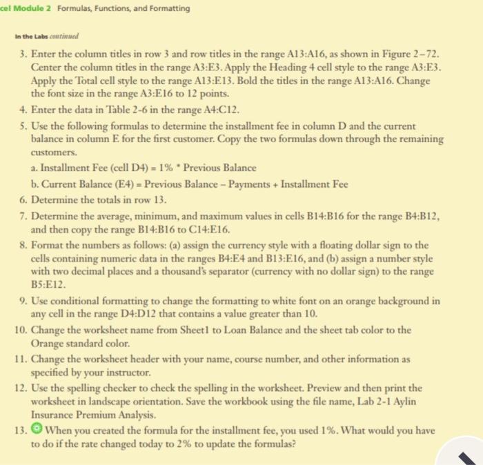
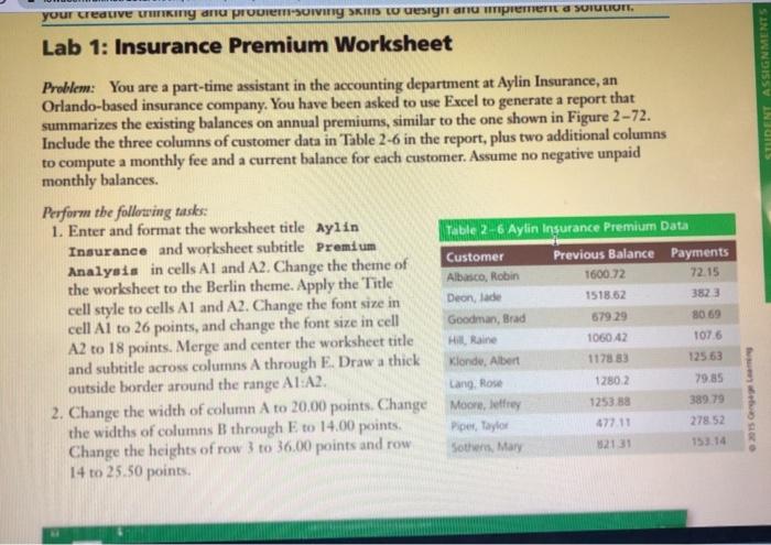
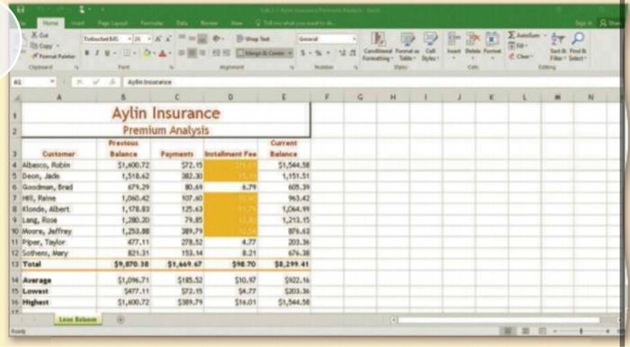
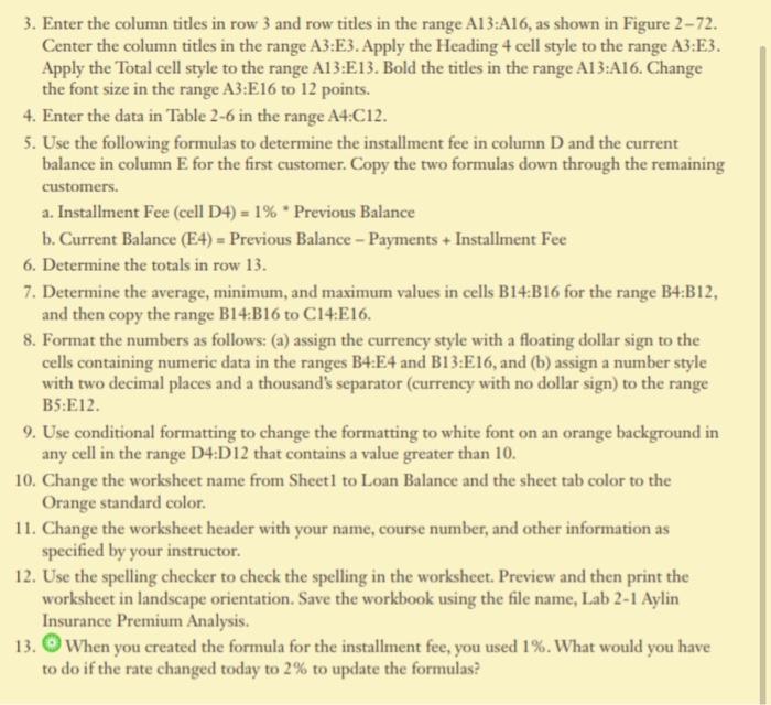
In the Labs Design, create, modify, and/or use a workbook following the guidelines concepts, and skills presented in this module. Labe 1 and 2 which increase in difficulty require you to create solutions based on what you leared in the moduleLab 3 requires you to apply your creative thinking and problem solving skills to design and element solution Lab 1: Insurance Premium Worksheet Pr. You are a part-time mistant in the accounting dance, Orlando-hued instance company Wou love been asked to weate a report that marines the casting balances en annual premiershwinan 2-72. Include the three column of medutain The-hewe will to computer monthly fee and a current balance for a construit monthly balance Refore the wing Enter and format the worksheet site ayita Insurance and worksheet beide Pream Analysis in cells. Al and A2. Change the theme of Previous Balance Payments the worksheet to the Berlin theme Apply the Tide cell style to cell Al A2. Change the fontein cell Alto 26 points, and can then call A2 to 18 points. Morge and center the whole and subtitle scrow columns A through E Drethik tid onder and the ALA! 2. Change the width of cum A to 20.00 points Change the width of column through 14.00 points Change the heaghts of roto 16.00 points and to 14 to 25.50 points . Aylin Insurance Figure 2-12 cel Module 2 Formulas, Functions, and Formatting In the Labe continued 3. Enter the column titles in row 3 and row titles in the range A13:416, as shown in Figure 272. Center the column titles in the range A3:E3. Apply the Heading 4 cell style to the range A3:E3. Apply the Total cell style to the range A13:E13. Bold the titles in the range A13:A16. Change the font size in the range A3:E16 to 12 points. 4. Enter the data in Table 2-6 in the range A4:C12. 5. Use the following formulas to determine the installment fee in column D and the current balance in column E for the first customer. Copy the two formulas down through the remaining customers. a. Installment Fee (cell D4) = 1% * Previous Balance b. Current Balance (E4) = Previous Balance - Payments + Installment Fee 6. Determine the totals in row 13. 7. Determine the average, minimum, and maximum values in cells B14:B16 for the range B4:B12, and then copy the range B14:B16 to C14:E16. 8. Format the numbers as follows: (a) assign the currency style with a floating dollar sign to the cells containing numeric data in the ranges B4:E4 and B13:E16, and (b) assign a number style with two decimal places and a thousand's separator (currency with no dollar sign) to the range B5:E12 9. Use conditional formatting to change the formatting to white font on an orange background in any cell in the range D4:D12 that contains a value greater than 10. 10. Change the worksheet name from Sheetl to Loan Balance and the sheet tab color to the Orange standard color. 11. Change the worksheet header with your name, course number, and other information as specified by your instructor. 12. Use the spelling checker to check the spelling in the worksheet. Preview and then print the worksheet in landscape orientation. Save the workbook using the file name, Lab 2-1 Aylin Insurance Premium Analysis. 13. When you created the formula for the installment fee, you used 1%. What would you have to do if the rate changed today to 2% to update the formulas? your creduve turiny dnu probleming SKI W Lesignanu mpement a solution. Lab 1: Insurance Premium Worksheet STUDENT ASSIGNMENTS Problem: You are a part-time assistant in the accounting department at Aylin Insurance, an Orlando-based insurance company. You have been asked to use Excel to generate a report that summarizes the existing balances on annual premiums, similar to the one shown in Figure 2-72. Include the three columns of customer data in Table 2-6 in the report, plus two additional columns to compute a monthly fee and a current balance for each customer. Assume no negative unpaid monthly balances. Perform the following tasks: 1. Enter and format the worksheet title Aylin Table 2-6 Aylin Insurance Premium Data Insurance and worksheet subtitle Premium Customer Previous Balance Payments Analysis in cells Al and A2. Change the theme of Albasco, Robin 1600.72 the worksheet to the Berlin theme. Apply the Title 72.15 Deon, lade 3823 cell style to cells AI and A2. Change the font size in cell A1 to 26 points, and change the font size in cell Goodman, Brad 679 29 80 69 A2 to 18 points. Merge and center the worksheet title Hill Rain 1060 42 TOT 6 and subtitle across columns A through E. Draw a thick Klonde, Albert 1178 83 12563 outside border around the range A1:A2. Lang, Rose 1280 2 79.85 2. Change the width of column A to 20.00 points. Change Moore, Jefrey 125388 389.79 the widths of columns B through E to 14.00 points Piper, Taylor 278 52 Change the heights of row 3 to 36.00 points and row Sothers, Mary 12131 14 to 25.50 points. 1518.62 153.14 WE gro H Aylin Insurance Premium Analysis Current HVIS Balance 51.600.73 912.15 bes, Robin Deontade red line Klode, Albert 51.544 1,151.51 05. . 10. 1,17 13.63 79.15 19 1,212.15 .. 203 More fry 11 per, Taylor 12 Soe, or 13 Total 21. 153. 20 38.2941 Average 15 Lowest Might $1.0.71 SAT.11 $122.1 510.0 54.71 598.01 $1,341.30 3. Enter the column titles in row 3 and row titles in the range A13:A16, as shown in Figure 2-72. Center the column titles in the range A3:E3. Apply the Heading 4 cell style to the range A3:E3. Apply the Total cell style to the range A13:E13. Bold the titles in the range A13:A16. Change the font size in the range A3:E16 to 12 points. 4. Enter the data in Table 2-6 in the range A4:C12. 5. Use the following formulas to determine the installment fee in column D and the current balance in column E for the first customer. Copy the two formulas down through the remaining customers. a. Installment Fee (cell D4) = 1% . Previous Balance b. Current Balance (E4) = Previous Balance - Payments + Installment Fee 6. Determine the totals in row 13. 7. Determine the average, minimum, and maximum values in cells B14:B16 for the range B4:B12, and then copy the range B14:B16 to C14:E16. 8. Format the numbers as follows: (a) assign the currency style with a floating dollar sign to the cells containing numeric data in the ranges B4:E4 and B13:E16, and (b) assign a number style with two decimal places and a thousand's separator (currency with no dollar sign) to the range B5:E12. 9. Use conditional formatting to change the formatting to white font on an orange background in any cell in the range D4:D12 that contains a value greater than 10. 10. Change the worksheet name from Sheetl to Loan Balance and the sheet tab color to the Orange standard color. 11. Change the worksheet header with your name, course number, and other information as specified by your instructor. 12. Use the spelling checker to check the spelling in the worksheet. Preview and then print the worksheet in landscape orientation. Save the workbook using the file name, Lab 2-1 Aylin Insurance Premium Analysis. 13. When you created the formula for the installment fee, you used 1%. What would you have to do if the rate changed today to 2% to update the formulas? In the Labs Design, create, modify, and/or use a workbook following the guidelines concepts, and skills presented in this module. Labe 1 and 2 which increase in difficulty require you to create solutions based on what you leared in the moduleLab 3 requires you to apply your creative thinking and problem solving skills to design and element solution Lab 1: Insurance Premium Worksheet Pr. You are a part-time mistant in the accounting dance, Orlando-hued instance company Wou love been asked to weate a report that marines the casting balances en annual premiershwinan 2-72. Include the three column of medutain The-hewe will to computer monthly fee and a current balance for a construit monthly balance Refore the wing Enter and format the worksheet site ayita Insurance and worksheet beide Pream Analysis in cells. Al and A2. Change the theme of Previous Balance Payments the worksheet to the Berlin theme Apply the Tide cell style to cell Al A2. Change the fontein cell Alto 26 points, and can then call A2 to 18 points. Morge and center the whole and subtitle scrow columns A through E Drethik tid onder and the ALA! 2. Change the width of cum A to 20.00 points Change the width of column through 14.00 points Change the heaghts of roto 16.00 points and to 14 to 25.50 points . Aylin Insurance Figure 2-12 cel Module 2 Formulas, Functions, and Formatting In the Labe continued 3. Enter the column titles in row 3 and row titles in the range A13:416, as shown in Figure 272. Center the column titles in the range A3:E3. Apply the Heading 4 cell style to the range A3:E3. Apply the Total cell style to the range A13:E13. Bold the titles in the range A13:A16. Change the font size in the range A3:E16 to 12 points. 4. Enter the data in Table 2-6 in the range A4:C12. 5. Use the following formulas to determine the installment fee in column D and the current balance in column E for the first customer. Copy the two formulas down through the remaining customers. a. Installment Fee (cell D4) = 1% * Previous Balance b. Current Balance (E4) = Previous Balance - Payments + Installment Fee 6. Determine the totals in row 13. 7. Determine the average, minimum, and maximum values in cells B14:B16 for the range B4:B12, and then copy the range B14:B16 to C14:E16. 8. Format the numbers as follows: (a) assign the currency style with a floating dollar sign to the cells containing numeric data in the ranges B4:E4 and B13:E16, and (b) assign a number style with two decimal places and a thousand's separator (currency with no dollar sign) to the range B5:E12 9. Use conditional formatting to change the formatting to white font on an orange background in any cell in the range D4:D12 that contains a value greater than 10. 10. Change the worksheet name from Sheetl to Loan Balance and the sheet tab color to the Orange standard color. 11. Change the worksheet header with your name, course number, and other information as specified by your instructor. 12. Use the spelling checker to check the spelling in the worksheet. Preview and then print the worksheet in landscape orientation. Save the workbook using the file name, Lab 2-1 Aylin Insurance Premium Analysis. 13. When you created the formula for the installment fee, you used 1%. What would you have to do if the rate changed today to 2% to update the formulas? your creduve turiny dnu probleming SKI W Lesignanu mpement a solution. Lab 1: Insurance Premium Worksheet STUDENT ASSIGNMENTS Problem: You are a part-time assistant in the accounting department at Aylin Insurance, an Orlando-based insurance company. You have been asked to use Excel to generate a report that summarizes the existing balances on annual premiums, similar to the one shown in Figure 2-72. Include the three columns of customer data in Table 2-6 in the report, plus two additional columns to compute a monthly fee and a current balance for each customer. Assume no negative unpaid monthly balances. Perform the following tasks: 1. Enter and format the worksheet title Aylin Table 2-6 Aylin Insurance Premium Data Insurance and worksheet subtitle Premium Customer Previous Balance Payments Analysis in cells Al and A2. Change the theme of Albasco, Robin 1600.72 the worksheet to the Berlin theme. Apply the Title 72.15 Deon, lade 3823 cell style to cells AI and A2. Change the font size in cell A1 to 26 points, and change the font size in cell Goodman, Brad 679 29 80 69 A2 to 18 points. Merge and center the worksheet title Hill Rain 1060 42 TOT 6 and subtitle across columns A through E. Draw a thick Klonde, Albert 1178 83 12563 outside border around the range A1:A2. Lang, Rose 1280 2 79.85 2. Change the width of column A to 20.00 points. Change Moore, Jefrey 125388 389.79 the widths of columns B through E to 14.00 points Piper, Taylor 278 52 Change the heights of row 3 to 36.00 points and row Sothers, Mary 12131 14 to 25.50 points. 1518.62 153.14 WE gro H Aylin Insurance Premium Analysis Current HVIS Balance 51.600.73 912.15 bes, Robin Deontade red line Klode, Albert 51.544 1,151.51 05. . 10. 1,17 13.63 79.15 19 1,212.15 .. 203 More fry 11 per, Taylor 12 Soe, or 13 Total 21. 153. 20 38.2941 Average 15 Lowest Might $1.0.71 SAT.11 $122.1 510.0 54.71 598.01 $1,341.30 3. Enter the column titles in row 3 and row titles in the range A13:A16, as shown in Figure 2-72. Center the column titles in the range A3:E3. Apply the Heading 4 cell style to the range A3:E3. Apply the Total cell style to the range A13:E13. Bold the titles in the range A13:A16. Change the font size in the range A3:E16 to 12 points. 4. Enter the data in Table 2-6 in the range A4:C12. 5. Use the following formulas to determine the installment fee in column D and the current balance in column E for the first customer. Copy the two formulas down through the remaining customers. a. Installment Fee (cell D4) = 1% . Previous Balance b. Current Balance (E4) = Previous Balance - Payments + Installment Fee 6. Determine the totals in row 13. 7. Determine the average, minimum, and maximum values in cells B14:B16 for the range B4:B12, and then copy the range B14:B16 to C14:E16. 8. Format the numbers as follows: (a) assign the currency style with a floating dollar sign to the cells containing numeric data in the ranges B4:E4 and B13:E16, and (b) assign a number style with two decimal places and a thousand's separator (currency with no dollar sign) to the range B5:E12. 9. Use conditional formatting to change the formatting to white font on an orange background in any cell in the range D4:D12 that contains a value greater than 10. 10. Change the worksheet name from Sheetl to Loan Balance and the sheet tab color to the Orange standard color. 11. Change the worksheet header with your name, course number, and other information as specified by your instructor. 12. Use the spelling checker to check the spelling in the worksheet. Preview and then print the worksheet in landscape orientation. Save the workbook using the file name, Lab 2-1 Aylin Insurance Premium Analysis. 13. When you created the formula for the installment fee, you used 1%. What would you have to do if the rate changed today to 2% to update the formulas