How do i complete the formula or references to populate the results for the data table with the ver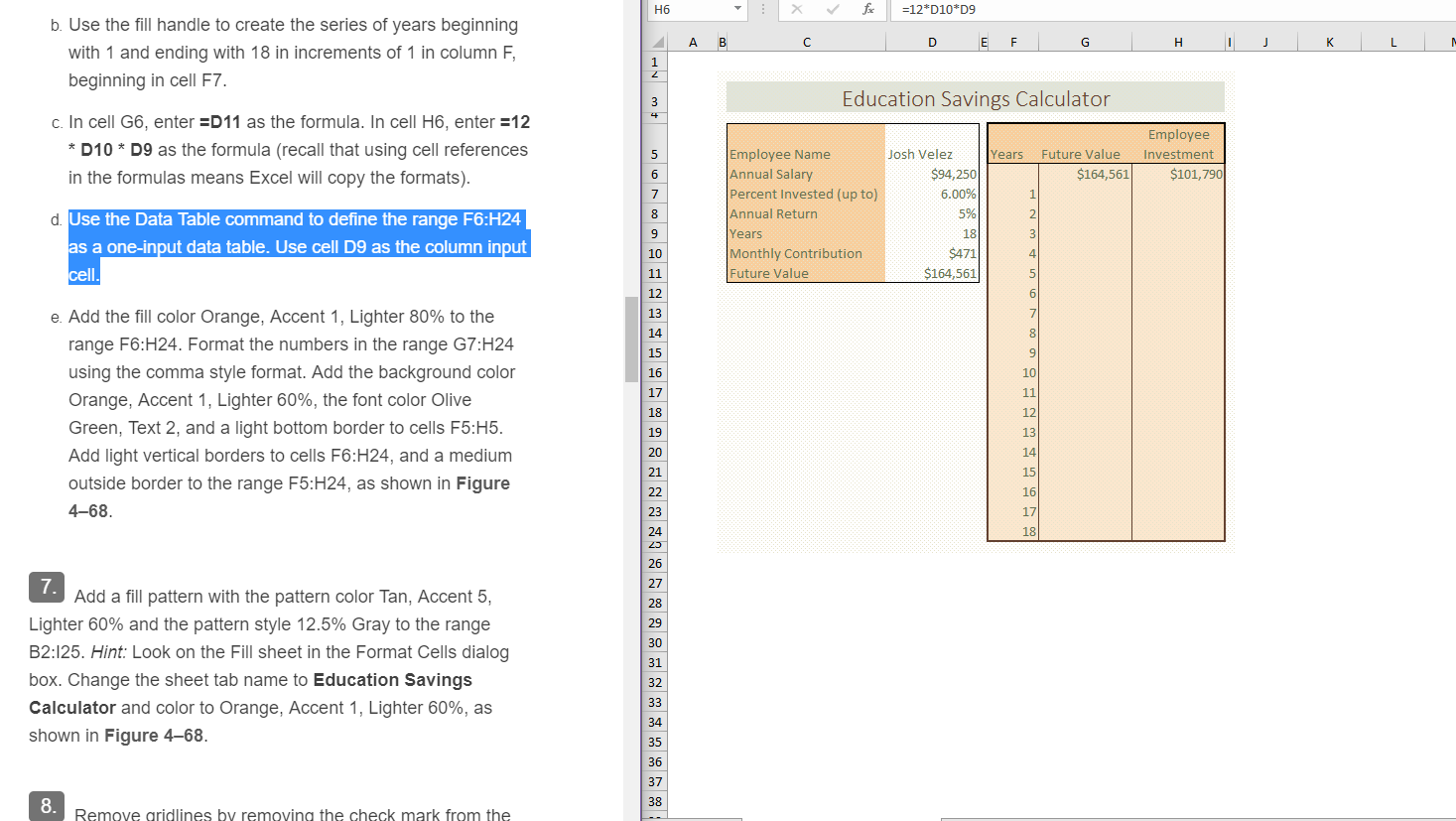tical values 1-18

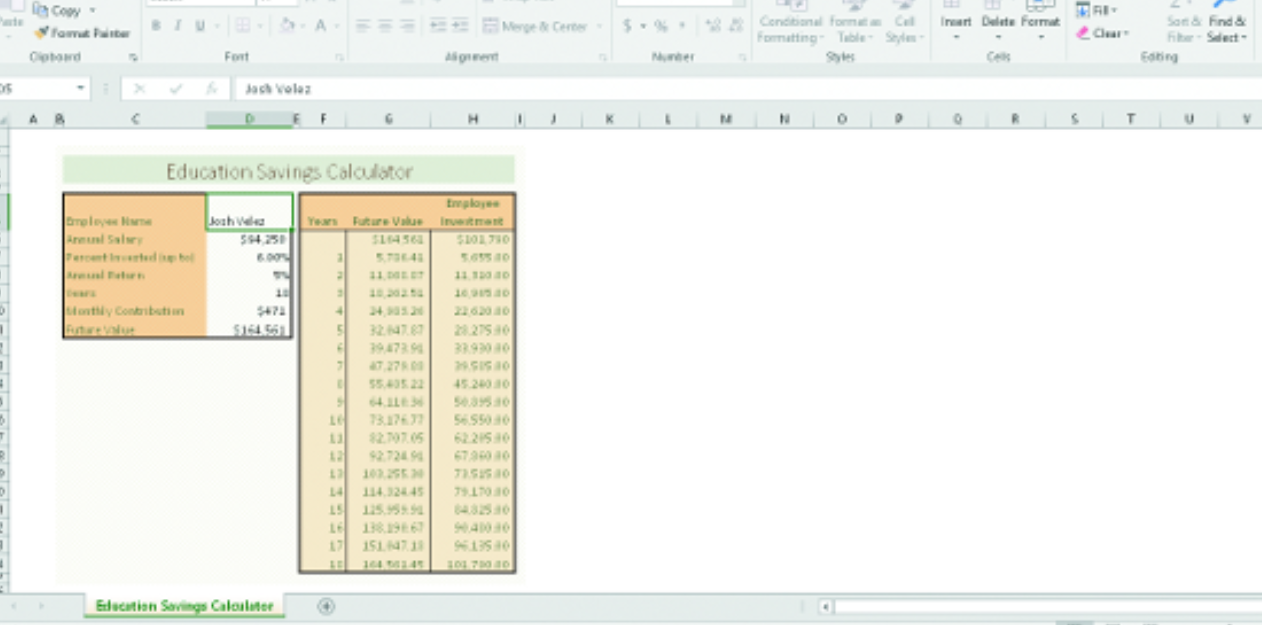
H6 =12*D10*D9 A B D E F G . J K L N b. Use the fill handle to create the series of years beginning with 1 and ending with 18 in increments of 1 in column F, beginning in cell F7. VAN + Education Savings Calculator c. In cell G6, enter =D11 as the formula. In cell H6, enter =12 * D10 * D9 as the formula (recall that using cell references in the formulas means Excel will copy the formats). 5 Years Josh Velez $94,250 6.00% Future Value $164,561 Employee Investment $101,790 6 7 8 Employee Name Annual Salary Percent Invested (up to) Annual Return Years Monthly Contribution Future Value 5% 9 d. Use the Data Table command to define the range F6:H24 as a one-input data table. Use cell D9 as the column input cell. 3 10 18 $471 $164,561 4 11 5. 12 6 13 7 14 8 15 9 10 11 17 e. Add the fill color Orange, Accent 1, Lighter 80% to the range F6:H24. Format the numbers in the range G7:H24 using the comma style format. Add the background color Orange, Accent 1, Lighter 60%, the font color Olive Green, Text 2, and a light bottom border to cells F5:H5. Add light vertical borders to cells F6:H24, and a medium outside border to the range F5:H24, as shown in Figure 468. 18 12 19 13 20 14 21 15 22 16 17 23 24 18 26 27 28 29 30 7. Add a fill pattern with the pattern color Tan, Accent 5, Lighter 60% and the pattern style 12.5% Gray to the range B2:125. Hint: Look on the Fill sheet in the Format Cells dialog box. Change the sheet tab name to Education Savings Calculator and color to Orange, Accent 1, Lighter 60%, as shown in Figure 468. 31 32 33 34 35 36 37 8. 38 Remove gridlines by removing the check mark from the Inat Duct Format Son Find & Le Coo low Coband 5. Conditional format Formatting Table Sale Nuwe Font Editing jach Volaz A F H 1 T Education Savings Calculator bosh va Arenal Predbe Employee Yes Future Value inima S11456 S1070 5610 11 DET 1110010 y Contribution 5 3287 2262010 250 22910 SES 10 1270 LE 56.500 622150 7355 10 T10 L 125 LE 1511 SIS Education Savings Calculator H6 =12*D10*D9 A B D E F G . J K L N b. Use the fill handle to create the series of years beginning with 1 and ending with 18 in increments of 1 in column F, beginning in cell F7. VAN + Education Savings Calculator c. In cell G6, enter =D11 as the formula. In cell H6, enter =12 * D10 * D9 as the formula (recall that using cell references in the formulas means Excel will copy the formats). 5 Years Josh Velez $94,250 6.00% Future Value $164,561 Employee Investment $101,790 6 7 8 Employee Name Annual Salary Percent Invested (up to) Annual Return Years Monthly Contribution Future Value 5% 9 d. Use the Data Table command to define the range F6:H24 as a one-input data table. Use cell D9 as the column input cell. 3 10 18 $471 $164,561 4 11 5. 12 6 13 7 14 8 15 9 10 11 17 e. Add the fill color Orange, Accent 1, Lighter 80% to the range F6:H24. Format the numbers in the range G7:H24 using the comma style format. Add the background color Orange, Accent 1, Lighter 60%, the font color Olive Green, Text 2, and a light bottom border to cells F5:H5. Add light vertical borders to cells F6:H24, and a medium outside border to the range F5:H24, as shown in Figure 468. 18 12 19 13 20 14 21 15 22 16 17 23 24 18 26 27 28 29 30 7. Add a fill pattern with the pattern color Tan, Accent 5, Lighter 60% and the pattern style 12.5% Gray to the range B2:125. Hint: Look on the Fill sheet in the Format Cells dialog box. Change the sheet tab name to Education Savings Calculator and color to Orange, Accent 1, Lighter 60%, as shown in Figure 468. 31 32 33 34 35 36 37 8. 38 Remove gridlines by removing the check mark from the