How do you do these steps into the excel sheet?

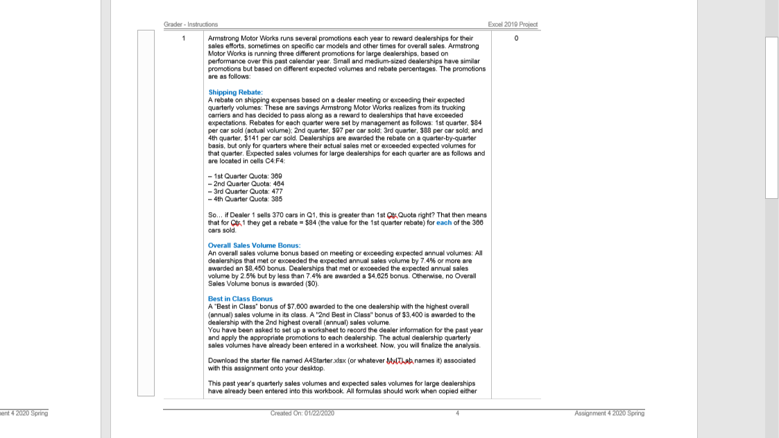
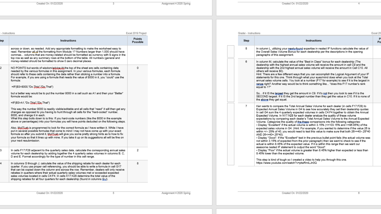
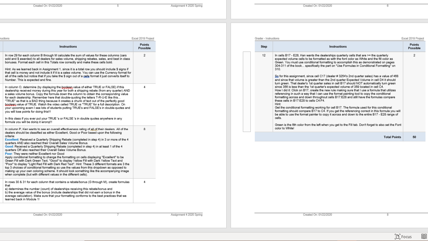
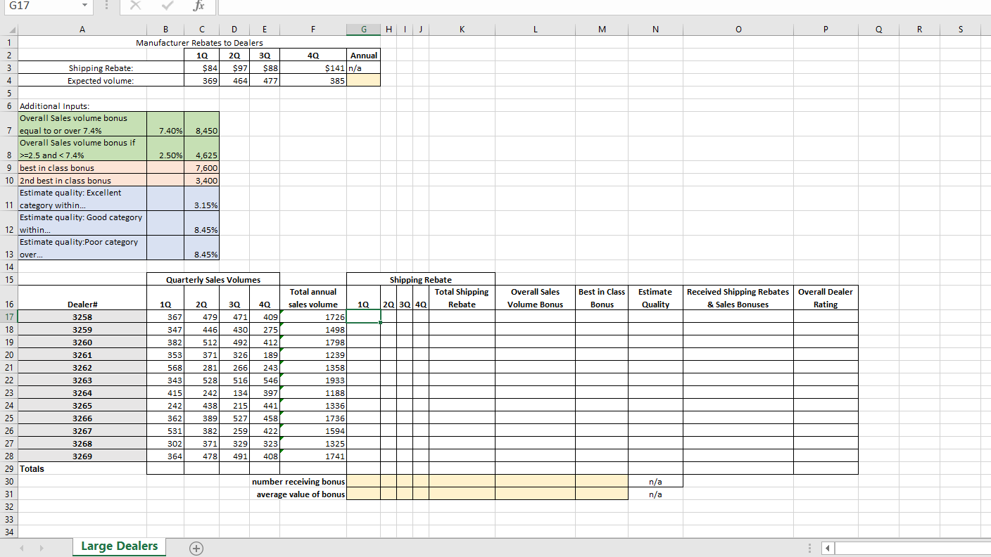
Grader - Instructions Expel 2019 Project Armstrong Motor Works runs several promotions each year to reward dealerships for their sales efforts, sometimes on specific car models and other times for overall sales. Armstrong Motor Works is running three different promotions for large dealerships, based on performance over this past calendar year, Small and medium-sized dealerships have similar promotions but based on different expected volumes and rebate percentages. The promotions are as follows Shipping Rebate: A rebate on shipping expenses based on a dealer meeting or exceeding their expected quarterly volumes: These are savings Armstrong Motor Works realizes from its trucking carriers and has decided to pass along as a reward to dealerships that have exceeded expectations, Rebates for each quarter were set by management as follows: 1st quarter, $84 per car sold (actual volume): 2nd quarter, $97 per car sold: 3rd quarter, $88 per car sold; and 4th quarter, $141 per car sold. Dealerships are awarded the rebate on a quarter-by-quarter basis, but only for quarters where their actual sales met or exceeded expected volumes for that quarter, Expected sales volumes for large dealerships for each quarter are as follows and are located in cells C4:F4: - 1st Quarter Quota: 369 - 2nd Quarter Quota: 464 - 3rd Quarter Quote: 477 - 4th Quarter Quota: 385 So.., if Dealer 1 sells 370 cars in Q1, this is greater than 1st Qtx Quota right? That then means that for Qt.1 they get a rebate = $84 (the value for the 1st quarter rebate) for each of the 380 cars sold. Overall Sales Volume Bonus: An overall sales volume bonus based on meeting or exceeding expected annual volumes: All dealerships that met or exceeded the expected annual sales volume by 7.4% or more are awarded an $8.450 bonus. Dealerships that met or exceeded the expected annual sales volume by 2.5% but by less than 7.4% are awarded a $4.625 bonus. Otherwise, no Overall Sales Volume bonus is awarded ($0). Best in Class Bonus A "Best in Class" bonus of $7.800 awarded to the one dealership with the highest overall (annual) sales volume in its class. A "2nd Best in Class" bonus of $3,400 is awarded to the dealership with the 2nd highest overall (annual) sales volume. You have been asked to set up a worksheet to record the dealer information for the past year and apply the appropriate promotions to each dealership. The actual dealership quarterly sales volumes have already been entered in a worksheet. Now, you will finalize the analysis. Download the starter file named A4Starter xlax (or whatever MylThat names it) associated with this assignment onto your desktop. This past year's quarterly sales volumes and expected sales volumes for large dealerships have already been entered into this workbook. All formulas should work when copied either ent 4 2020 Spring Created On: 01/2272020 Assignment 4 2020 SpringCreated On: 01/22/2020 Assignment 4 2020 Spring Created On: 01/22/2020 - Instructions Excel 2019 Project Grader - Instructions Expel 2 tep Instructions Points Possible Step Instructions Po across or down, as needed. Add any appropriate formatting to make the worksheet easy to 5 In column L. utilizing your newly-found expertise in nested IF functions calculate the value of read. Remember all of the formatting from Module 1? Numbers larger than 1.000 should have the Overall Sales Volume Bonus for each dealership per the descriptions in the opening commas... columns that are money-related should be formatted as currency with $ signs in the paragraphs of this assignment top row as well as any summary rows at the bottom of the table. All numbers (general and money-related should be formatted to show 0 zero decimal places. In column M, calculate the value of the "Best in Class" bonus for each dealership (The dealership with the highest annual sales volume will receive the amount in cell CO and the NO POINTS but words of wisdom/advice At the top of the sheet are cells containing data needed by the various formulas in this assignment. In your various formulas, each formula dealership with the 2nd highest annual sales volume will receive the amount in Cell C10. All should refer to these cells containing the data rather than sticking a number into a formula. others will receive $0). For example, if you are using a formula that needs the value of 8000 in it, you "could" use the Hint: There are a few different ways that you can accomplish the Logical Argument of your IF statements for this one. Think through what your eyes/mind does when you look at the Total formula: annual sales volume cells. You look at a number (F17 for example) to see if it is the largest in =IF(83>8000,"Do This\\"Do That") equal to 1?" range right? Another way would be to think something like... "does this F17 number's rank but a better way would be to put the number 8000 in a cell such as A1 and then your "Better" So... if it IS the largest they get the amount in CO. If it's not then you look to see if it is the formula would be: SECOND largest. If it IS the 2nd largest number than they get the value in C10. If it is none of the above they get squat. =IF(83>A1,"Do This""Do That") 7 This way the number 8000 is readily visible/editable and all cells that "need" it will then get any Ken wants to compare the Total Annual Sales Volume for each dealer (in cells F17:F28) to Expected Annual Sales Volume in 34 to see how accurately they set their dealership quotas: changes as opposed to you having to hunt through all cells for the "hard-coded" number, 8000, and change it in each. In cell G4 sum the 4 quarterly expected volumes in cells C4:F4 together to obtain the Annual What this step boils down to is this: If you hard-code numbers (like the 8000 in the example Expected Volume. In N17:N28 for each dealer analyze the quality of these volume above or percentages) into your formulas you will have points deducted on the following steps. expectations by comparing each dealer's Total Annual Sales Volume to the Annual Expected Volume. Categorize the quality of the these comparisons into the following categories: Also. MyThat is programmed to look for the correct formula as I have written it. While I have . Display "Excellent" if the actual volume is within 3. 15% (=06.85%) of the put in several possible formulas that come to mind I may not have come up with your exact expected sales volume in G4. (Hint: For example, if you wanted to determine if the value 26 is formula so after you submit it. My(That will give you some pretty strong hints as to how to fix within +/- 25% of 40, you would need to test this value to make sure that both 26>=40-,25*40 your formula so that it lines up with mine. If you take it up on its suggestions all will be fine on AND 26= the quarterly expected volume cells to be formatted as with the font color as White and the fill color as bonuses. Format each cell in this Totals row correctly and make these cells bold. Green. You must use conditional formatting to accomplish this as demonstrated on pages Hint: As we learned back in Assignment 1. since it is a total row you should include $ signs if 304-311 of the book... specifically the part on "Use Formulas in Conditional Formatting" on 310 that cell is money and not include it if it is a sales volume. You can use the Currency format for all of the cells but notice that if you take the $ sign out of a calls format it just converts itself to So for this assignment, since cell C17 (dealer # 3254's 2nd quarter sales) has a value of 468 Number, This is expected and fine. and since that volume is greater than the 2nd quarter Expected Volume in cell D4 it should In column O, determine (by displaying the boolegg value of either TRUE or FALSE) if this turn green. That dealer's 1st quarter sales in cell B17 should NOT automatically turn green dealership received money during this year for both a shipping rebate (from any quarter) AND since 356 is less than the 1st quarter's expected volume of 350 located in cell C4. a sales volume bonus, Copy the formula down the column to obtain the corresponding value How I did it: Click on B17, create the new rule making sure that I use a formula that utilizes for each dealership. Remember here that double-quoting the letters T-R-U-E like this.. referencing in such a way that I can use the format painting tool to copy the conditional 'TRUE" as that is a BAD thing because it creates a chunk of text out of the perfectly good formatting across and down throughout cells B17:E28 and still have the formulas compare these cells in B17:E28 to cells C4:F4. boolean value of TRUE. Watch the video called TRUE vs "TRUE" for a full description. On your upooming exam I see lots of students putting TRUE's and FALSE's in double-quotes and Hint: Get the conditional formatting working for cell B17. The formula used for this conditional you will lose points for doing this! formatting should compare $17 to C4. If you get the referencing correct in this formula you will cells . be able to use the format painter to copy it across and down to the entire B17 - E28 range of In this class if you ever put your TRUE's or FALSE's in double quotes anywhere in any formula you will be doing it wrong! In column P, Ken wants to see an overall effectiveness rating of all of their dealers. All of the color to White! Green is the Oth color from the left when you get to the Fil tab. Don't forget to also set the Font dealers should be classified as either Excellent. Good or Poor based upon the following criteria Excellent: Received a Quarterly Shipping Rebate (completed in step 4) in 3 or more of the 4 Total Points 50 quarters AND also reached their Overall Sales Volume Bonus. Good: Received a Quarterly Shipping Rebate (completed in step 4) in at least 1 of the 4 quarters OR also reached their Overall Sales Volume Bonus. Poor: They were neither Excellent nor Good Apply conditional formatting to change the formatting on cells displaying "Excellent" to be Green Fill with Dark Green Text, "Good" to display Yellow Fill with Dark Yellow Text and "Poor" to display "Light Red Fill with Dark Red Text". Hint: These 3 different formats are 3 the top 3 choices of conditional formatting so use the values from this dropdown as opposed to making up your own coloring scheme. It should look something like the accompanying image when complete (but with different values in the different cells) In rows 30 & 31 for each column that contains a rebate/bonus (G through M). create formulas that a) determines the number (count) of dealerships receiving this rebate/bonus and b) the average value of the bonus (include dealerships that did not earn a bonus in the average calculation). Make sure that your formatting conforms to the best practices that we learned back in Module 1! Created On: 01/22/2020 Assignment 4 2020 Spring Created On: 01/22/2020 " FocusG17 X Jx A B C D E F G H I J K L M N O P Q R S Manufacturer Rebates to Dealers AWN 10 20 30 40 Annual Shipping Rebate: $84 $97 $88 $141 n/a Expected volume: 369 464 477 385 un 6 Additional Inputs Overall Sales volume bonus 7 equal to or over 7.4% 7.40% 8.450 Overall Sales volume bonus if 8 >=2.5 and