How to determine whether it is normally distributed since they look skewed.

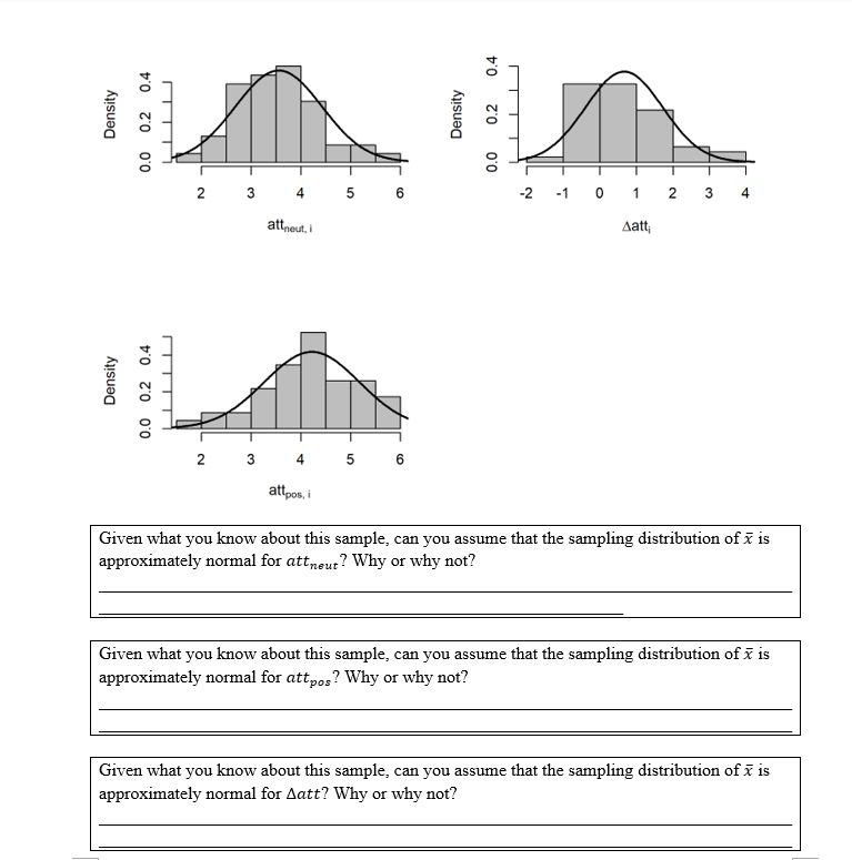
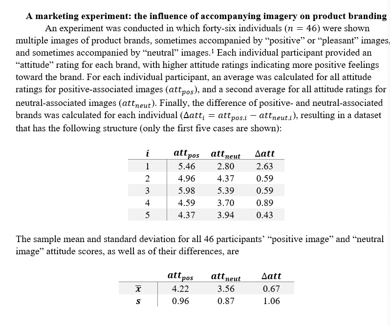
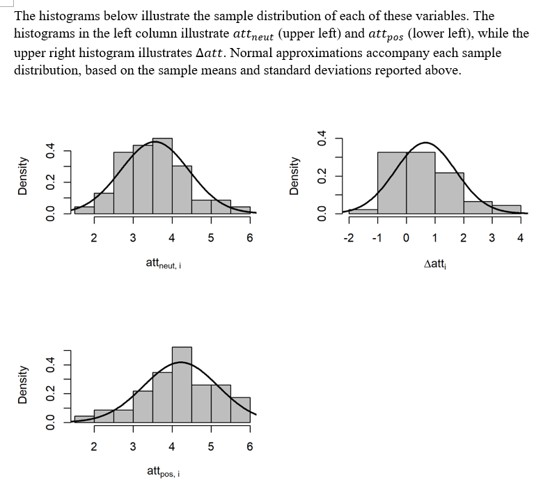
Dansin Density 0.0 0.2 0.4 Dansin 0.0 0.2 0.4 Given what you know about this sample, can you assume that the sampling distribution of i is approximately normal for attmt? Why or why not? Given what you know about this sample, can you assume that the sampling distribution of i is appmximately normal for arty\"? Why or why not? Given what you know about this sample, can you assume that the sampling distribution of i is approximately normal for att? Why or why not? A marketing experiment: the inuence of accompanying imagery on product branding An experiment was conducted in which forty-six individuals (n = 46) were shown multiple images of product brands, sometimes accompanied by \"positive" or \"pleasant" images, and sometimes accompanied by \"neutr \" images.1 Each individual participant provided an \"attitude" rating for each brand, with higher attitude ratings indicating more positive feelings toward the brand. For each individual participant, an average was calculated for all attitude ratings for positive-associated images (attpas), and a second average for all attitude ratings for neutral-associated images (attnwt). Finally, the difference of positive- and neutral-associated brands was calculated for each individual (Autti = attposli attmu\"), resulting in a dataset that has the following structure {only the rst ve cases are shown): 1' art1m can\"; anti 1 5.46 2.80 2.63 2 4.96 4.31r 0.59 3 5.98 5.39 0.59 4 5 4.59 3.?0 0.89 437 3.94 0.43 3|\". The sample mean and standard deviation for all 46 participants positive image\" and \"neutral image" attitude scores, as well as of their differences, are at: as grim,\" Autt i 4.22 3.56 0.6? s 0.96 0.8? 1.06 m The histograms below illustrate the sample distribution of each of these variables. The histograms in the left column illustrate attneut (upper left) and attpos (lower left), while the upper right histogram illustrates dart. Normal approximations accompany each sample distribution, based on the sample means and standard deviations reported above. Density Density 0.0 0.2 0.4 Density 0.0 0.2 0.4