i = 10%, g = 2%, N =16, Discount 3 periods, use geometric gradient series formula

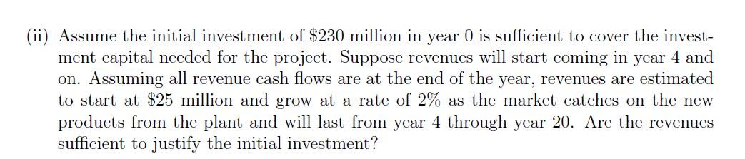
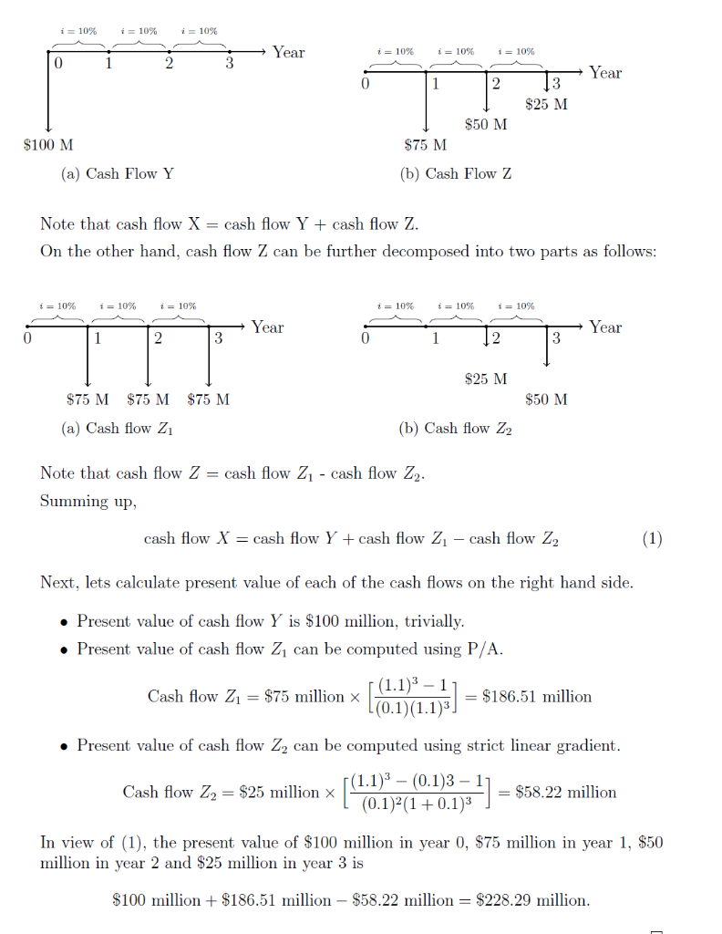
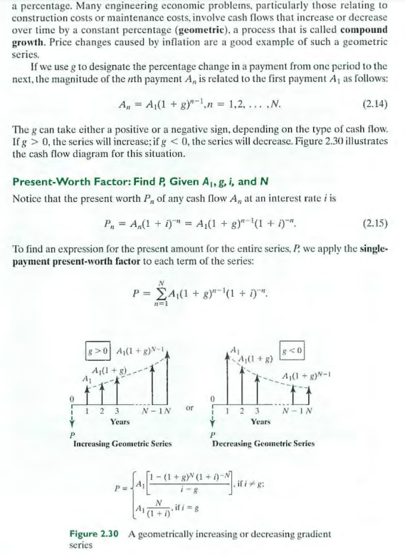
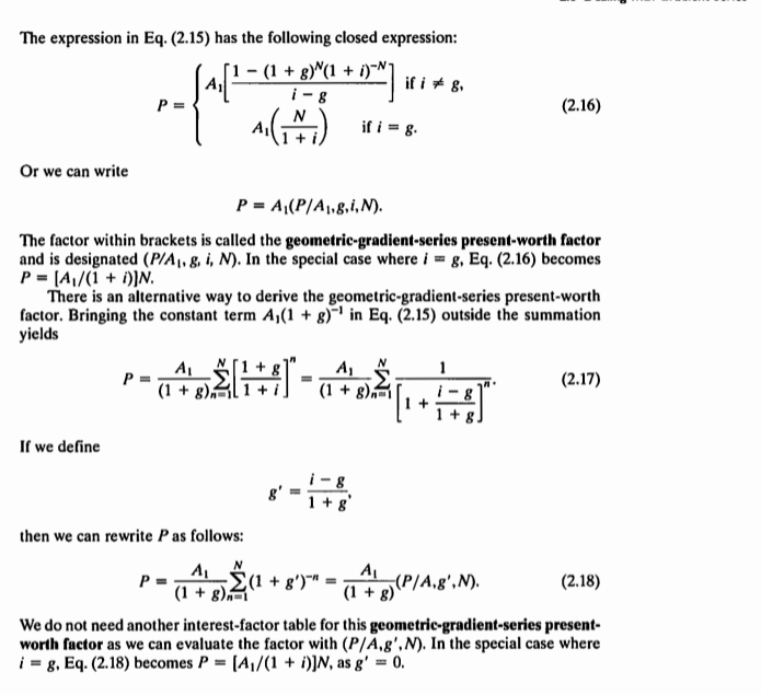
(ii) Assume the initial investment of $230 million in year 0 is sufficient to cover the invest- ment capital needed for the project. Suppose revenues will start coming in year 4 and on. Assuming all revenue cash flows are at the end of the year, revenues are estimated to start at $25 million and grow at a rate of 2% as the market catches on the new products from the plant and will last from year 4 through year 20. Are the revenues sufficient to justify the initial investment? i = 10% i = 10% i = 10% Year i = 10% i= 10% i = 10% 0 3 Year 3 $25 M $50 M $100 M $75 M (a) Cash Flow Y (b) Cash Flow Z Note that cash flow X = cash flow Y + cash flow Z. On the other hand, cash flow Z can be further decomposed into two parts as follows: i = 10% i = 10% = 10% i= 10% i = 10% i = 10% Year Year 0 1 2 3 0 1 2 3 $25 M $75 M $75 M $75 M $50 M (a) Cash flow Z (b) Cash flow Z2 Note that cash flow Z = cash flow 21 - cash flow Z. Summing up cash flow X = cash flow Y + cash flow Z1 - cash flow Z2 (1) Next, lets calculate present value of each of the cash flows on the right hand side. Present value of cash flow Y is $100 million, trivially. Present value of cash flow Z can be computed using P/A. Cash flow Z1 = $75 million x (1.1)3 - 1 (0.1)(1.1) = $186.51 million Present value of cash flow Z2 can be computed using strict linear gradient. Cash flow Z2 = $25 million (1.1)3 (0.1)3 - 1 (0.1)-(1 +0.13 H] = $58.22 million In view of (1), the present value of $100 million in year 0, $75 million in year 1, $50 million in year 2 and $25 million in year 3 is $100 million + $186.51 million - $58.22 million = $228.29 million. a percentage. Many engineering economic problems, particularly those relating to construction costs or maintenance costs, involve cash flows that increase or decrease over time by a constant percentage (geometric), a process that is called compound growth. Price changes caused by inflation are a good example of such a geometric series. If we use g to designate the percentage change in a payment from one period to the next, the magnitude of the nth payment A, is related to the first payment A, as follows: A = A (1 + g)"-In = 1,2. ... .N. (2.14) The g can take either a positive or a negative sign, depending on the type of cash flow. Ifg > 0, the series will increase; if g 04/(1+ g)N- A(1+) A(1+) 1,(1 + + g)-1 0 1 2 3 Years N-IN or N-IN Years P P Increasing Geometric Series Decreasing Geometrie Series - (1 + g) (1 + i)-N7 A) 1990 + 0 +7 N 4! (1 + i) Figure 2.30 A geometrically increasing or decreasing gradient series The expression in Eq. (2.15) has the following closed expression: (1 - (1 + 8)^(1 + i)-N7 if i 8, i-g P= N Ja[ (2.16) Or we can write P = A (P/A1,8,1,N). The factor within brackets is called the geometric-gradient-series present-worth factor and is designated (P/A, 8, 1, N). In the special case where i = g, Eq. (2.16) becomes P = (1/(1 + i)]N. There is an alternative way to derive the geometric-gradient-series present-worth factor. Bringing the constant term A,(1 + 8) in Eq. (2.15) outside the summation yields A Ai 1 (2.17) (1 + 8) (1 + 8). [+1- If we define i-8 O then we can rewrite P as follows: A Pa AL *(1 + 8')" (2.18) (1 + 8). (1 + 8) We do not need another interest-factor table for this geometric-gradient-series present- worth factor as we can evaluate the factor with (P/A,8',N). In the special case where i = g, Eq. (2.18) becomes P = (1/(1 + i)]N, as g' = 0. (P/4,8'.M). (ii) Assume the initial investment of $230 million in year 0 is sufficient to cover the invest- ment capital needed for the project. Suppose revenues will start coming in year 4 and on. Assuming all revenue cash flows are at the end of the year, revenues are estimated to start at $25 million and grow at a rate of 2% as the market catches on the new products from the plant and will last from year 4 through year 20. Are the revenues sufficient to justify the initial investment? i = 10% i = 10% i = 10% Year i = 10% i= 10% i = 10% 0 3 Year 3 $25 M $50 M $100 M $75 M (a) Cash Flow Y (b) Cash Flow Z Note that cash flow X = cash flow Y + cash flow Z. On the other hand, cash flow Z can be further decomposed into two parts as follows: i = 10% i = 10% = 10% i= 10% i = 10% i = 10% Year Year 0 1 2 3 0 1 2 3 $25 M $75 M $75 M $75 M $50 M (a) Cash flow Z (b) Cash flow Z2 Note that cash flow Z = cash flow 21 - cash flow Z. Summing up cash flow X = cash flow Y + cash flow Z1 - cash flow Z2 (1) Next, lets calculate present value of each of the cash flows on the right hand side. Present value of cash flow Y is $100 million, trivially. Present value of cash flow Z can be computed using P/A. Cash flow Z1 = $75 million x (1.1)3 - 1 (0.1)(1.1) = $186.51 million Present value of cash flow Z2 can be computed using strict linear gradient. Cash flow Z2 = $25 million (1.1)3 (0.1)3 - 1 (0.1)-(1 +0.13 H] = $58.22 million In view of (1), the present value of $100 million in year 0, $75 million in year 1, $50 million in year 2 and $25 million in year 3 is $100 million + $186.51 million - $58.22 million = $228.29 million. a percentage. Many engineering economic problems, particularly those relating to construction costs or maintenance costs, involve cash flows that increase or decrease over time by a constant percentage (geometric), a process that is called compound growth. Price changes caused by inflation are a good example of such a geometric series. If we use g to designate the percentage change in a payment from one period to the next, the magnitude of the nth payment A, is related to the first payment A, as follows: A = A (1 + g)"-In = 1,2. ... .N. (2.14) The g can take either a positive or a negative sign, depending on the type of cash flow. Ifg > 0, the series will increase; if g 04/(1+ g)N- A(1+) A(1+) 1,(1 + + g)-1 0 1 2 3 Years N-IN or N-IN Years P P Increasing Geometric Series Decreasing Geometrie Series - (1 + g) (1 + i)-N7 A) 1990 + 0 +7 N 4! (1 + i) Figure 2.30 A geometrically increasing or decreasing gradient series The expression in Eq. (2.15) has the following closed expression: (1 - (1 + 8)^(1 + i)-N7 if i 8, i-g P= N Ja[ (2.16) Or we can write P = A (P/A1,8,1,N). The factor within brackets is called the geometric-gradient-series present-worth factor and is designated (P/A, 8, 1, N). In the special case where i = g, Eq. (2.16) becomes P = (1/(1 + i)]N. There is an alternative way to derive the geometric-gradient-series present-worth factor. Bringing the constant term A,(1 + 8) in Eq. (2.15) outside the summation yields A Ai 1 (2.17) (1 + 8) (1 + 8). [+1- If we define i-8 O then we can rewrite P as follows: A Pa AL *(1 + 8')" (2.18) (1 + 8). (1 + 8) We do not need another interest-factor table for this geometric-gradient-series present- worth factor as we can evaluate the factor with (P/A,8',N). In the special case where i = g, Eq. (2.18) becomes P = (1/(1 + i)]N, as g' = 0. (P/4,8'.M)