

Question: i nedd help with data entry in excel DATA ENTERY IN EXCELL I was looking for someone who can enter the information provided in excel.
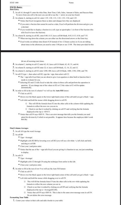
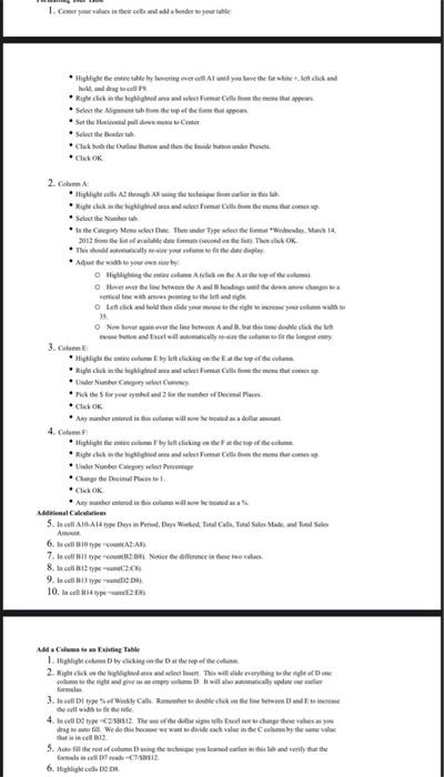
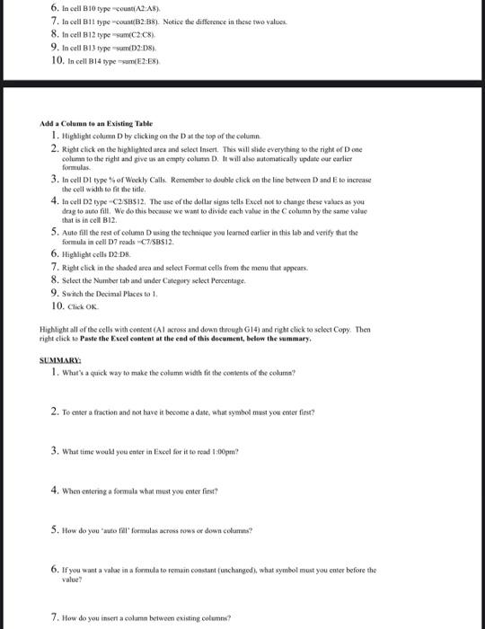
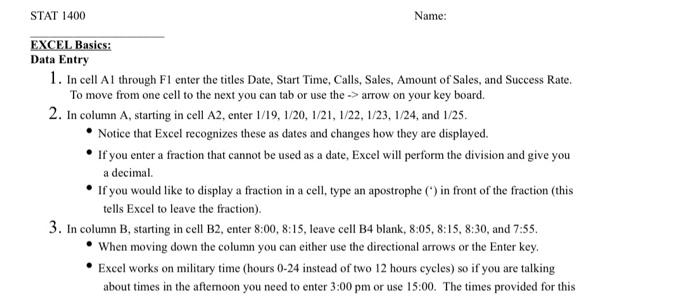

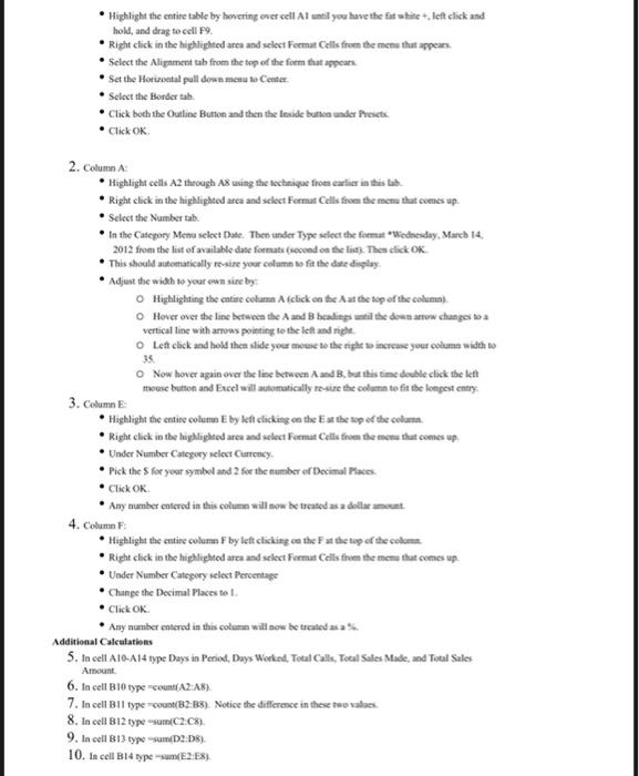
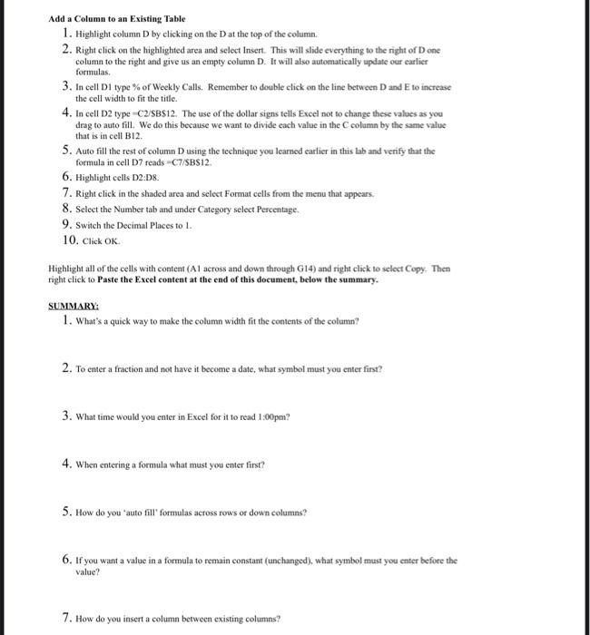
STATO Nam EXCEL Data Tatry 1. la cell At through Fl enter the title Date Start Time, Calle, Sales, Sole Sec Rate To from the meat you can tabarche a your keyboard 2. In cuma starting in cell 18.12.131.122.1/24, 121/23 Notice that comes the date and charges how they are deplaseid yeterince we will performed give your demel you would like to deploy and specification the contract 3. le cabine Bating cente....well B4 105 82,55 homing det helmeye cather was the theme key Excelenty time has 0.34 instead of why you weg shemes in the after you need to mer 100 w 500 The times prided for the label 4. Incolume Curtig indster 62.41, kuve cell Cuk,62,45,51,64 5. Incolas D. starting in cellente 22.6, le cell, 12.121 and 12 6. Incore unting leter 200,480. ledl 4 bln. 1400, 150, 239, and 7. Incl 2 type o scored 12. type thesis, then clon C2 The will see that you get the built in fact that neede elf you Selecting and tells Fixed take the title cells perlim hepen question danger of the values in the se in 2 will be dete utically 8. In order to de rest of wilt Auto Fille Click to Hver ever the black square in the lower right hand mere his edl stilou petak Lait dick wallet This will find the funds for the other cells in the same while printer formularelect the way in O Check to see that worked by chcel Fund verifying the female dupled the pics Notice that cells. This was atemor message that lets you the formula you well and for den by which is the appears became the employed that may Find Column Average 1. to call the word 2.9 Type Bible will see ik wil and drag te Cluse your pre Notice that the designere you are giving action to watching dile 3. to call Type * Highlight palace throat any the techanics team are the tah, Cand prompt 4.toder total in the roof we will use the store Click Hover the black square in the weight become a cell til you per a lack Let ick and the modern vertelle The will fill the same from whether the inter while doing the recewcolm you Check to see that it worked by clicking on cell and verifying that the forma dupled the topic o See that all PV This was the mergemine Des de dorm Formatting Voer 1. Centeryer values in their ladda border to your 1. hrist Hulighetene by hoveringer Aliyoshehehe.lendid oldal .Righteome Celle om te me that Select the line from the perfelpen +la theriammal - tran Select the Click bort the end CULOK 2.Com light Actor * Pipithelaalalaalaal Cela tami cette er * In the Cape Menschen der Type de la desde 14 2012 The OK The call in your mother play Highlighting them in the mi line edhe line between Abending and there was a verticale with and o ludikohen did you here your womew 25 Overgavere line between Abstinenteil w and or will be they 3. Cum * Highlight come by Wiking the top al die Une Number nyerhelderheim *CK . Any usher della Higiene come by to clicking the top om ' Rahat near tirighted are anslation farmers the lem Underwear . Deci est CHOK All Cities 5. od 16 A14 type Days in Penal Day Wed Thu Cat. Tol Sales Made Tools 6. Il 10 AZAD to e Bleo No he different move 8. In cell 12type- 9. tecell B13) 10. In Hype Add Coming Table 1.lightlome Deco 2. Right ce dle This will see the in the right not put tatata mental 3.ltype Weekly Calle de se ne 4. e cell 252 The wheat siges Exchange there as you Ing. We do this www divide each valori lub tem valor 5. Althie foto coming the children that she find ca. 6. Belightede 2.0 6. la cell B10 type A2:48) 7. In cell B11 type-count/B2: B8). Notice the difference in these two values 8. In cell B12 type mc2.c), 9. In cell B13 type sum 02:08 10. In cell B14 type sumE2:28) Add a Column to an Existing Table 1. Highlight column D by clicking on the Dat the top of the column 2. Right lick on the highlighted area and select Insert. This will slide everything to the right of Done column to the right and give us an empty column D. It will also automatically update our earlier formulas 3. In cell Dl types of Weekly Calls. Remember to double click on the line between D and Eto increase the cell width to fit the tide, 4. In cell D2 typeC258512. The use of the dollar signs tells Exed not to change these values as you drag to auto fill. We do this because we want to divide each value in the column by the same value that is in cell B12 5. Auto fill the rest of column D using the technique you learned earlier in this lab and verify that the formula in cell D7 reads -C/SBS12. 6. Highlight cells 12DB 7. Right click in the shaked area and select Format cells from the menu that appears. 8. Select the Number tab and under Catepory select Percentage 9. Switch the Decimal Places to I 10. Click OK Highlight all of the cells with content (Al across and down through G14) and right click to select Copy. Then right click to Paste the Excel content at the end of this document, below the summary, SUMMARY: 1. What's a quick way to make the column width fit the contents of the colima? 2. To enter a fraction and not have it become a date, What symbol must you enter tirse? 3. What time would you enter in Excel for it to road 1:00pm! 4. When entering a formula what must you enter first? 5. How do you "auto fill formulas across tows or down columu? 6. If you want a value in a formula to remain constant (unchanged), what symbol must you enter before the value 7. How do you insert a column between existing columta? STAT 1400 Name: EXCEL Basies: Data Entry 1. In cell Al through Fl enter the titles Date, Start Time, Calls, Sales, Amount of Sales, and Success Rate. To move from one cell to the next you can tab or use the -> arrow on your key board. 2. In column A, starting in cell A2, enter 1/19,1/20, 1/21, 1/22, 1/23, 1/24, and 1/25 Notice that Excel recognizes these as dates and changes how they are displayed. If you enter a fraction that cannot be used as a date, Excel will perform the division and give you a decimal. If you would like to display a fraction in a cell, type an apostrophe () in front of the fraction (this tells Excel to leave the fraction). 3. In column B, starting in cell B2, enter 8:00, 8:15, leave cell B4 blank, 8:05, 8:15, 8:30, and 7:55. When moving down the column you can either use the directional arrows or the Enter key, Excel works on military time (hours 0-24 instead of two 12 hours cycles) so if you are talking about times in the aftemoon you need to enter 3:00 pm or use 15:00. The times provided for this automatically lab are all morning (am) times. 4. In column C, starting in cell Center 62. 43, leave cell C blank. 62.45.31, and 64. 5. In column D, starting in cell D2 enter 22, 6. leave cell D4 blank, 12, 16, 22, and 12 6. In column E, starting in cell E2 enter 1200, 480, leave cell 4 blank, 1400, 1356, 2380, and 750. 7. In cell F2 type then select cell D2, type the sign, then select cell C2. The sign tells Excel that you are about to give it an equation or other built in function that it needs to evaluate for you Selecting D2 and C2 tells Excel to take the values in those cells and perform the operation in question. If you change one of the values in 2 or C2 the value in F2 will be update 8. In order to fill in the rest of column F we will use the Auto Fill feature: Click in cell F2 Hover over the black square in the lower right hand corner of this cell until you get a black + sign. Lett click and hold the mouse while dragging down to cell F8 This will fill the formula from F2 into the other cells in the column while updating the formula to reflect the new row you are in o Check to see that it worked by clicking on cell FS and verifying that the formula displayed at the top is-DSCS. Notice that cell 4 sayx #DIV/0. This is an error message that tells you the formula you used asked for division by O which is not possible. It appears here because the employee didn't work that day. Find Column Averages 1. In cell A9 type the word Average 2. In cell B9 Type -Average Highlight colls B2-B8 by hovering over cell B2 (you will see a fut write + left click and hold. and drag to cell B Close your ) and press enter Notice that the use of the = sign tells Excel you are giving it a function to use, not just something to display 3. In cell c9 Type =Averaget Highlight cells C2 through C using the technique from carlier in this lab. Close your ) and press enter 4. In order to fill in the rest of row 9 we will use the Auto Fill feature Click in cell c. Hover over the black square in the lower right hand comer of this cell until you get a black + sign Left click and hold the mouse while dragging over to cell 9 This will fill the formula from C9 into the other cells in the row while updating the formula to reflect the new column you are in Check to see that it worked by clicking on cell D9 and verifying that the formula displayed at the top is --AverageD2D8% O Notice that cell P9 says WDIV/0. This is due to the same error message seen in cell F4. Do not delete this error message Formatting Your Table 1. Center your values in their cells and add a border to your table: Highlight the entire table by hovering over cell Al until you have the fat white + lef click and hold, and drag to cell 19. Right click in the highlighted area and select Format Cells from the menu that appears Select the Alignment tab from the top of the form that appears * Set the Horizontal pull down menu to Center Select the Border tah. Click both the Outline Buton and then the Inside better under Presete Click OK 35 2. Column Highlight cells A2 through A8 wing the technique from earlier in this lab. Right click in the highlighted area and select Format Cells from the menu that comes up Select the Number tab In the Category Menu sclect Date. Then under Type select the format Wednesday, March 14. 2012 from the list of available date formats second on the list. The dick OK This should automatically resire your column to fit the date display Adjust the width to your own site by Highlighting the entire column A (click on the Aat the top of the column) Hover over the line between the A and B headings until the downtow changes a vertical line with arrows pointing to the left and right o Lett click and hold the slide your mouse to the right increase your column width to Now hover again over the line between A and B. but this time double click the lett mouse button and Excel will automatically resize the column to fit the longest entry 3. Column Highlight the entire column E by kft clicking co the Es the top of the columns Right click in the highlighted area and select Format Cells from the menu that comes up Under Number Category select Currency Pick the for your symbol and for the number of Decimal Places Click OK Any namber entered in this column will now be treated as a della ment 4. Column Highlight the entire column F by lett clicking ces the Fat the top of the colom Right click in the highlighted area and select Format Cells from the menu that comes up, Under Number Category select Percentage Change the Decimal Places to Click OK Any number entered in this columns will now be treated as Additional Calculations 5. In cell A10-A14 type Days in Period, Days Worked. Total Calls, Total Sales Made, and Total Sales 6. In cell B10 type count(A2-AB). 7. In cell Bil type count(B2:88). Notice the difference in these two values 8. In cell B12 typesum(C2.08) 9. In cell B13 type-samD2:08). 10. In cell B14 type sum(E2:EX) Amount Add a Column to an Existing Table 1. Highlight column D by clicking on the Dat the top of the column. 2. Right click on the highlighted area and select Insert. This will slide everything to the right of Done column to the right and give us an empty column D. It will also automatically update our earlier formulas. 3. In cell D1 type of Weekly Calls. Remember to double click on the line between D and to increase the cell width to fit the title. 4. In cell D2 type-C2/B$12. The use of the dollar signs tells Excel not to change these values as you drag to auto fill. We do this because we want to divide each value in the column by the same value that is in cell B12. 5. Auto fill the rest of column D using the technique you learned earlier in this lab and verify that the formula in cell D7 reads C7/8BS12. 6. Highlight cells 02:08 7. Right click in the shaded area and select Format cells from the menu that appears. 8. Select the Number tab and under Category select Percentage 9. Switch the Decimal Places to L. 10. Click OK Highlight all of the cells with content (Al across and down through G14) and right click to select Copy. Then right click to Paste the Excel content at the end of this document, below the summary. SUMMARY: 1. What's a quick way to make the column width fit the contents of the column? 2. To enter a fraction and not have it become a date, what symbol must you enter first? 3. What time would you enter in Excel for it to read 1:00pm? 4. When entering a formula what must you enter first? 5. How do you auto fill formulas across rows or down columns? 6. If you want a value in a formula to remain constant (unchanged), what symbol must you enter before the value? 7. How do you insert a column between existing columns
Step by Step Solution
There are 3 Steps involved in it

Get step-by-step solutions from verified subject matter experts